System and Method for Non-Invasive Buried Pipe Condition Assessment Using Surface-Mounted Vibro-Acoustic Sensor Arrays and Physics-Informed Graph Neural Networks

Abstract

Disclosed is a system and method for assessing the structural condition of buried water distribution pipes without excavation or internal inspection. The system deploys arrays of surface-mounted piezoelectric accelerometers at existing above-ground access points (fire hydrants, valve boxes, meter pits) and uses controlled vibro-acoustic excitation to propagate guided elastic waves through pipe walls. A physics-informed graph neural network (PI-GNN) ingests the recorded waveforms alongside a topological model of the pipe network, jointly inferring pipe material classification, wall thickness estimation, corrosion grade, and remaining useful life for each pipe segment. The physics-informed loss function encodes the Pochhammer-Chree dispersion relations for cylindrical waveguides, constraining the neural network to produce physically consistent predictions even with sparse sensor coverage. The system reduces per-segment assessment cost from $5,000-15,000 (excavation-based) to under $200, enabling utilities to survey entire distribution networks within a single budget cycle.

Field of the Invention

This invention relates to non-destructive evaluation of underground utility infrastructure, specifically to the use of surface-accessible vibro-acoustic sensing combined with physics-constrained machine learning for condition assessment of buried water distribution pipes.

Background

The United States operates approximately 2.2 million miles of water distribution pipe (EPA 7th Drinking Water Infrastructure Needs Survey, 2023). The ASCE 2025 Infrastructure Report Card grades U.S. drinking water infrastructure at C-, unchanged from 2021. An estimated 260,000 water main breaks occur annually in the U.S. and Canada (Utah State University Buried Structures Laboratory, 2024), at an estimated remediation and social cost exceeding $2.6 billion per year.

A critical obstacle to proactive pipe replacement is condition uncertainty. Utilities typically know pipe diameter, approximate installation date, and nominal material for only 60-70% of their networks (AWWA Research Foundation, Condition Assessment Strategies). For the remainder, records are incomplete or missing entirely. Current condition assessment methods include:

• Excavation and direct inspection: The gold standard, but costs $5,000-15,000 per test pit depending on depth, surface restoration, and traffic control. Provides condition data for a single point on a single pipe. Impractical for system-wide assessment.
• Internal inspection (CCTV, smart pigging): Requires pipe dewatering or insertion of in-line tools. Applicable primarily to transmission mains (12"+ diameter). Cost: $15-40 per linear foot. Not feasible for small-diameter distribution mains (4"-8") that constitute 80%+ of network length.
• Acoustic leak detection: Correlators such as the Sewerin AQUAPHON and Echologics LeakFinderST use acoustic propagation velocity to estimate average pipe wall thickness between two access points. Effective for leak localization but provides only bulk-average condition over the full segment, missing localized corrosion.
• Statistical break prediction: Models such as those described by Scheidegger et al., J. Infrastructure Systems 2015 predict break probability from age, material, soil type, and historical break records. Useful for capital planning but cannot identify specific segments needing replacement and systematically underperform for pipes with no break history.

The gap in the art is a non-invasive, cost-effective method that: (a) assesses individual pipe segment condition from the surface without excavation or dewatering, (b) identifies pipe material when utility records are missing, (c) provides spatially resolved wall thickness and corrosion estimates rather than segment averages, and (d) integrates network-wide data through a topology-aware model that propagates information from instrumented segments to uninstrumented neighbors.

Detailed Description

1. Sensor Hardware and Deployment

The system uses industrial-grade piezoelectric accelerometers (e.g., PCB Piezotronics 352C33, sensitivity 100 mV/g, frequency range 0.5-10,000 Hz, resonant frequency 50 kHz) mounted via magnetic clamps to exposed metallic pipe fittings at fire hydrants, valve stems, and meter pit risers. For non-metallic fittings, epoxy-bonded mounting pads provide acoustic coupling.

Each sensor node comprises: the accelerometer; a 24-bit analog-to-digital converter (e.g., Texas Instruments ADS1256, 30 kSPS) for high dynamic range; a microcontroller (e.g., STM32L4 series, ARM Cortex-M4 with FPU) for local signal conditioning and buffering; a LoRa radio module (Semtech SX1262) or LTE-M cellular modem for data backhaul; a rechargeable lithium battery (3.7V, 6000 mAh) with solar trickle charger; and a weatherproof IP67 enclosure. Target per-node bill-of-materials cost: $180-250.

2. Vibro-Acoustic Excitation

Controlled acoustic excitation is applied at selected access points using one of two methods:

• Electromagnetic shaker: A portable electromagnetic actuator (e.g., modified from The Modal Shop K2007E01) is clamped to a fire hydrant barrel and driven with a chirp signal sweeping 50-5,000 Hz over 10 seconds. Peak force: 45 N. The chirp provides broadband excitation that illuminates all guided wave modes within the frequency band of interest.
• Controlled valve operation: A rapid partial closure (20-50 ms) of a gate valve generates a pressure transient that couples into pipe wall vibration. This method requires no additional equipment but produces less repeatable excitation.

The excitation generates guided elastic waves that propagate along the pipe wall. In a fluid-filled cylindrical shell, the dominant propagating modes are: the L(0,1) longitudinal mode (compressional wave along pipe axis, group velocity 1,000-5,200 m/s depending on material and frequency); the L(0,2) mode (higher-order longitudinal, typically above 2 kHz cutoff for 6" cast iron); the F(1,1) flexural mode (bending wave, dispersive, group velocity 200-1,500 m/s); and the T(0,1) torsional mode (non-dispersive in uniform pipe, velocity determined solely by shear modulus).

3. Signal Processing Pipeline

Raw accelerometer data is sampled at 20 kHz with 24-bit resolution. The processing pipeline applies: band-pass filtering (30-8,000 Hz, 8th-order Butterworth) to reject DC offset, 60 Hz power line interference, and high-frequency sensor resonance artifacts; short-time Fourier transform (STFT) with 2048-sample Hann window and 75% overlap, producing a time-frequency representation at 2.44 Hz frequency resolution and 25.6 ms time resolution; dispersion curve extraction via the phase-shift method (Park et al., Geophysics 1999), computing frequency-dependent phase velocity from cross-spectral analysis between sensor pairs; and arrival time picking using an Akaike Information Criterion (AIC) autopicker (Maeda, BSSA 1985) for each identified wave mode.

The processed output for each excitation event is a feature tensor containing: the empirical dispersion curve (phase velocity vs. frequency) for each detected mode; the group velocity for each mode; spectral attenuation coefficients (dB/m vs. frequency); and arrival times and amplitudes at each receiving sensor.

4. Physics-Informed Graph Neural Network

The core inference engine is a graph neural network (GNN) whose graph structure mirrors the physical pipe network topology. Nodes represent instrumented access points (hydrants, valves, meters). Edges represent pipe segments connecting adjacent nodes. The GNN architecture uses a message-passing framework (Gilmer et al., ICML 2017) with the following structure:

• Node features (input): GPS coordinates, elevation, local soil resistivity (from USDA SSURGO database), groundwater depth, surface traffic loading category, and sensor measurement summary statistics.
• Edge features (input): Pipe diameter (from GIS records, or 6" default when unknown), segment length, installation year (when known, or zero-encoded when missing), nominal material (one-hot encoded, with an "unknown" class), number of historical breaks on this segment, and the full feature tensor from vibro-acoustic measurements.
• Hidden layers: 6 message-passing layers with 256-dimensional hidden state, using gated recurrent update functions. Edge attention weights (4-head attention) allow the model to weight information from adjacent segments differently based on measurement quality and topological context.
• Output (per edge): Pipe material classification (cast iron, ductile iron, steel, PVC, HDPE, asbestos cement, concrete cylinder, unknown); estimated wall thickness profile (mean and standard deviation, in mm); corrosion condition grade (1-5 scale aligned with NASSCO PACP structural grading); and estimated remaining useful life (years, with 80% confidence interval).

5. Physics-Informed Loss Function

The GNN training loss comprises three terms:

Data fidelity loss (L_data): Mean squared error between predicted and measured dispersion curves, arrival times, and attenuation profiles at instrumented segments. This term is active only at edges with sensor data.

Physics residual loss (L_physics): The model's predicted material properties (density ρ, Young's modulus E, Poisson's ratio ν) and wall thickness (h) for each segment are fed into the Pochhammer-Chree frequency equation for a fluid-filled cylindrical waveguide. The residual of this dispersion relation, evaluated at 50 frequency points across the measurement bandwidth, is penalized. Specifically, for the L(0,1) mode, the phase velocity c_p at angular frequency ω must satisfy:

det[M(c_p, ω, ρ, E, ν, h, a, ρ_f, c_f)] = 0

where M is the 6×6 coefficient matrix from the Pochhammer-Chree derivation, a is the pipe inner radius, ρ_f is the fluid density, and c_f is the fluid sound speed. The physics loss penalizes the squared magnitude of this determinant when evaluated at the model's predicted parameters and the measured (c_p, ω) pairs. This constrains predictions to be physically realizable even at uninstrumented edges where no measurement data exists.

Graph smoothness loss (L_smooth): A regularization term penalizing large discontinuities in predicted condition grade between adjacent pipe segments of the same material and similar age, reflecting the physical prior that corrosion conditions are spatially correlated along a pipe run.

Total loss: L = L_data + λ_p · L_physics + λ_s · L_smooth, with hyperparameters λ_p = 0.1 and λ_s = 0.01 determined via cross-validation on a held-out utility dataset.

6. Training Data and Transfer Learning

The model is pre-trained on synthetic data generated by a finite-element pipe model (e.g., COMSOL Multiphysics Structural Mechanics module) simulating guided wave propagation in pipes of varying material, diameter (4"-24"), wall thickness (3-25 mm), and corrosion profiles (uniform thinning, pitting, graphitic corrosion in cast iron). The synthetic dataset comprises 500,000 simulated excitation-response pairs across 12 pipe material classes and 50 corrosion severity levels.

Fine-tuning uses field data from partnering utilities that have performed excavation-based condition assessment alongside vibro-acoustic measurements at the same locations. A minimum of 200 ground-truth validated segments across 3+ pipe materials is required for effective transfer to a new utility's network. The model architecture supports continual learning: each new excavation provides a labeled training sample that refines predictions for the surrounding network region.

7. Edge Deployment and Continuous Monitoring

For initial survey mode, a field crew visits each access point once, installs a temporary sensor, triggers an excitation event, records 30 seconds of response data, and moves to the next node. A crew of two can instrument 40-60 nodes per day, surveying 10-15 miles of distribution network.

For continuous monitoring mode, permanently installed sensor nodes record ambient vibration from traffic loading, water hammer events, and pump cycling. The GNN processes ambient data in 24-hour batches, updating condition estimates without active excitation. Continuous monitoring enables detection of acute condition changes (e.g., a new crack or joint displacement) within 48 hours of onset, triggering an alert to the utility's asset management system via REST API webhook.

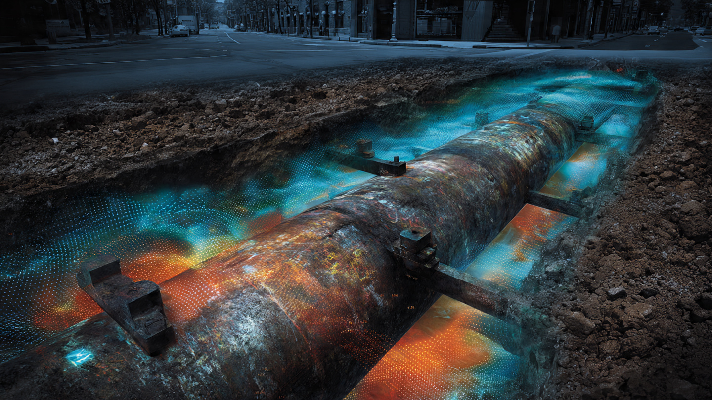
8. Figures Description

• Figure 1: System architecture showing the pipe network graph with sensor nodes at hydrants and valves, data flow from field sensors through the signal processing pipeline to the PI-GNN, and output condition assessment dashboard.
• Figure 2: Dispersion curves (phase velocity vs. frequency) for four common pipe materials (cast iron, ductile iron, PVC, HDPE) at nominal and corroded wall thicknesses, showing the discriminating features used by the classifier.
• Figure 3: Graph neural network message-passing architecture, showing how information propagates from instrumented nodes to uninstrumented neighbors over 6 layers, with attention-weighted edge updates.
• Figure 4: Network-wide condition assessment heatmap for a representative 50-mile distribution zone, with color-coded pipe segments showing predicted remaining useful life and flagged critical segments.

Claims

1. A system for non-invasive condition assessment of buried water distribution pipes, comprising: a plurality of surface-mounted vibro-acoustic sensor nodes deployed at above-ground pipe access points; an excitation source that generates controlled elastic waves propagating through pipe walls; and a physics-informed graph neural network that receives recorded waveform data and a topological model of the pipe network, and outputs per-segment condition assessments including material classification, wall thickness estimation, and remaining useful life prediction.
2. The system of claim 1, wherein the graph neural network encodes the pipe network as a graph with nodes at instrumented access points and edges representing pipe segments, and uses message-passing layers to propagate condition information from instrumented segments to uninstrumented neighboring segments.
3. The system of claim 1, wherein the physics-informed loss function constrains the neural network's material property and wall thickness predictions to satisfy the Pochhammer-Chree dispersion relations for guided elastic waves in fluid-filled cylindrical shells.
4. The system of claim 1, wherein the signal processing pipeline extracts empirical dispersion curves from cross-spectral analysis between sensor pairs, and the dispersion curve shape serves as a discriminating feature for pipe material classification.
5. The system of claim 1, further comprising a continuous monitoring mode wherein permanently installed sensor nodes record ambient vibration from traffic, water hammer, and pump cycling, and the graph neural network updates condition estimates without active excitation.
6. A method for assessing buried pipe condition comprising: deploying vibro-acoustic sensors at above-ground pipe access points across a water distribution network; applying controlled acoustic excitation and recording guided wave responses; extracting frequency-dependent phase velocity, group velocity, and attenuation features from the recorded signals; constructing a graph representation of the pipe network topology; and training a physics-informed graph neural network to jointly infer pipe material, wall thickness, corrosion grade, and remaining useful life for each pipe segment.
7. The method of claim 6, wherein the model is pre-trained on synthetic guided wave data generated by finite-element simulation of pipes with varying material, diameter, wall thickness, and corrosion profiles, and fine-tuned on field measurements validated against excavation-based ground truth.
8. The method of claim 6, further comprising a graph smoothness regularization term that penalizes discontinuities in predicted condition grade between adjacent pipe segments of similar material and age, encoding the physical prior that corrosion is spatially correlated.
9. The method of claim 6, wherein pipe material is classified from dispersion curve shape, exploiting the distinct phase velocity vs. frequency signatures of cast iron, ductile iron, steel, PVC, HDPE, and asbestos cement pipes.
10. The system of claim 1, wherein each sensor node has a bill-of-materials cost below $300 and is deployable at fire hydrants, valve boxes, and meter pits without excavation, pipe dewatering, or traffic control measures.

Prior Art References

1. EPA 7th Drinking Water Infrastructure Needs Survey, 2023 — 2.2 million miles of U.S. water distribution pipe
2. ASCE 2025 Infrastructure Report Card — C- grade for drinking water
3. Utah State University Buried Structures Laboratory, 2024 — 260,000+ annual water main breaks, $452B funding gap
4. AWWA Research Foundation — Condition assessment strategies and practices for water mains
5. Scheidegger et al., J. Infrastructure Systems 2015 — Statistical pipe break prediction models
6. Echologics (Mueller Water Products) — Acoustic pipe wall assessment technology
7. PCB Piezotronics 352C33 — ICP accelerometer for vibration measurement
8. Park et al., Geophysics 1999 — Phase-shift method for dispersion curve extraction
9. Maeda, BSSA 1985 — AIC autopicker for seismic arrival time detection
10. Gilmer et al., ICML 2017 — Message Passing Neural Networks
11. NASSCO PACP — Pipeline Assessment and Certification Program structural grading
12. COMSOL Multiphysics — Finite element simulation for guided wave modeling
13. Muggleton et al., Applied Sciences 2020 — Comprehensive review of acoustic methods for locating underground pipelines
14. Li et al., Sensors 2022 — Three-dimensional localization of buried polyethylene pipes using acoustic methods