System and Method for Non-Invasive Classification of Buried Water Service Line Materials and Condition Assessment Using Vehicle-Mounted Multi-Frequency Electromagnetic Induction Arrays, Ground-Penetrating Radar, and Deep Learning Material Fingerprinting
Abstract
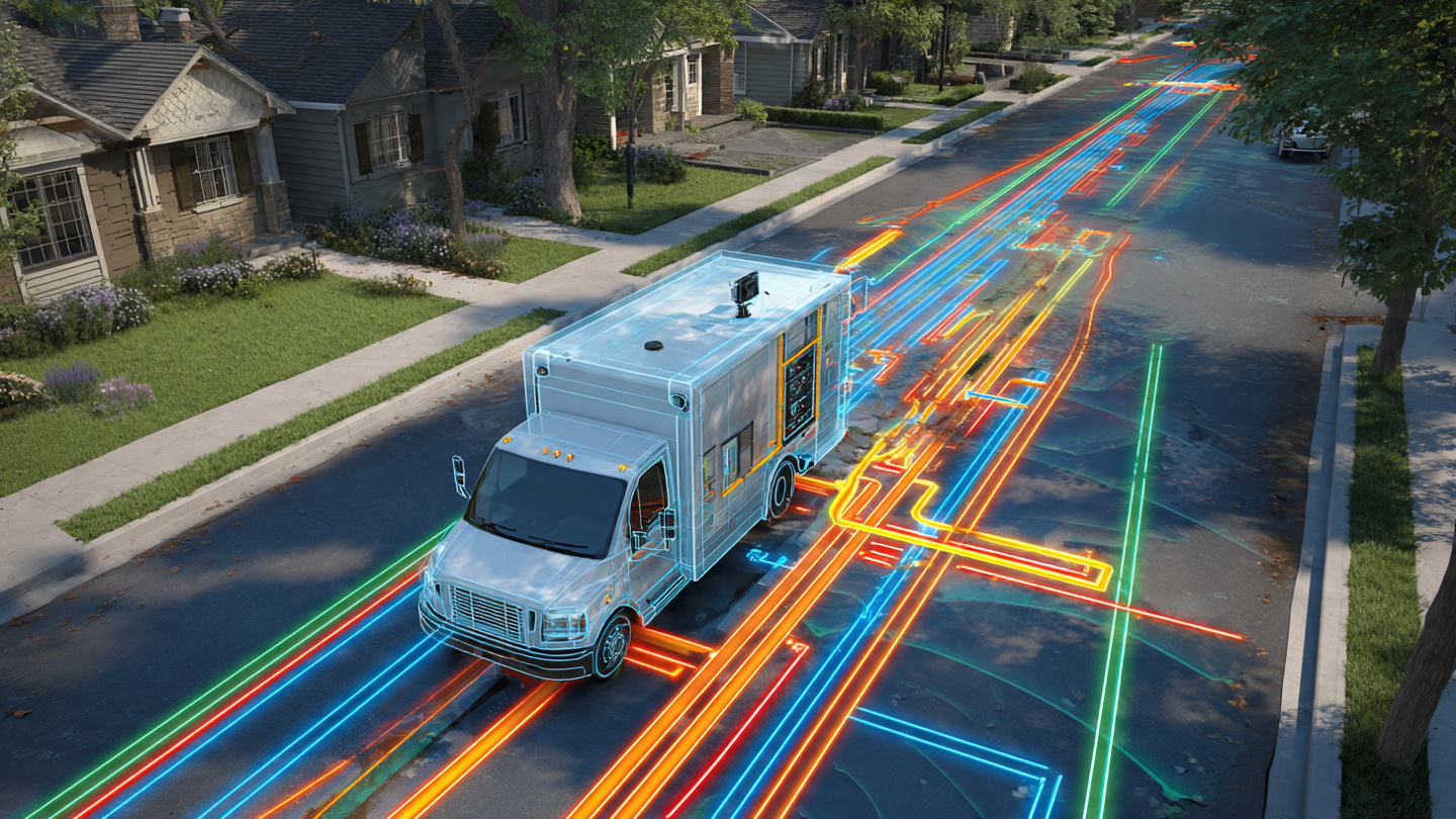
Disclosed is a system and method for non-invasive identification and condition assessment of buried water service lines using sensor arrays mounted on routine utility fleet vehicles. The system combines multi-frequency electromagnetic induction (EMI) sensing at 6 discrete frequencies spanning 1 kHz to 100 kHz with vehicle-mounted ground-penetrating radar (GPR) operating at 800 MHz and 1.6 GHz center frequencies. EMI response signatures differ systematically across service line materials: lead pipes exhibit high conductivity (4.8 × 10⁶ S/m) with negligible magnetic permeability (μᵣ ≈ 1), producing strong in-phase response with minimal quadrature at all frequencies; galvanized steel shows moderate conductivity (5.8 × 10⁶ S/m for the zinc coating, 1.0 × 10⁷ S/m for the steel substrate) combined with high relative permeability (μᵣ ≈ 200-1,000), generating frequency-dependent phase rotation; copper exhibits the highest conductivity (5.96 × 10⁷ S/m) with no ferromagnetic response; ductile iron combines high permeability (μᵣ ≈ 100-500) with moderate conductivity; and PVC generates no electromagnetic response, identifiable by GPR reflection alone. A convolutional neural network processes fused EMI phase-quadrature spectrograms and GPR B-scan radargrams to classify pipe material with target accuracy exceeding 92%, estimate nominal pipe diameter (½″, ¾″, 1″, 1¼″, 2″), and infer wall condition from corrosion-induced conductivity degradation profiles. The system operates at normal driving speeds of 15-25 mph, processes data on-board via edge GPU, and uploads classified segments with GPS coordinates to a GIS database for utility asset management and regulatory compliance with the EPA Lead and Copper Rule Revision.
Field of the Invention
This invention relates to subsurface utility infrastructure characterization, specifically to the non-invasive identification of buried water service line materials and condition assessment using vehicle-mounted electromagnetic induction and ground-penetrating radar sensor fusion with machine learning classification.
Background
The United States has approximately 9.2 million lead service lines connecting water mains to residential buildings (EPA estimate, 2024). The revised Lead and Copper Rule (LCRR), finalized October 2024, requires all water systems to complete a comprehensive service line inventory by October 2027, classifying every service line as lead, galvanized requiring replacement, or non-lead. Systems with lead service lines must replace them within 10 years. The Biden-Harris administration allocated $15 billion from the Bipartisan Infrastructure Law specifically for lead service line replacement, with an additional $11.7 billion in EPA Drinking Water State Revolving Fund financing. The American Water Works Association estimated total national replacement costs at $60 billion.
The fundamental challenge is not replacement itself but identification: most water utilities do not know what their service lines are made of. A 2016 AWWA survey found that 40% of utilities had incomplete or no records of service line material. Many pre-1950 water systems maintained paper records that have been lost, damaged, or never digitized. The LCRR's inventory deadline has forced utilities into a massive identification campaign under severe time pressure.
Current service line material identification methods have critical limitations:
- Records review: Searching historical plumbing permits, tap cards, and meter installation records. Cheapest approach ($5-15 per line) but incomplete; Michigan's statewide inventory found records could classify only 38% of service lines with confidence.
- Physical excavation ("potholing"): Digging to expose the pipe at the property line. Definitive identification but costs $500-3,000 per address and takes 30-60 minutes of crew time. At 9.2 million lead lines nationwide (and roughly 100 million total service lines needing classification), full excavation would cost $50-300 billion and take decades.
- Predictive modeling: Statistical models using building age, neighborhood demographics, and historical plumbing practices to predict material likelihood. Trueman et al. (Environmental Science & Technology, 2021) achieved 74-85% accuracy, insufficient for regulatory compliance which requires "verifiable" identification.
- Interior inspection: Scratching exposed pipe at the water meter or building entry point with a coin (lead is soft and silvery; copper is hard and reddish). Requires interior access to every building, homeowner coordination, and only identifies the interior portion. The service line material may differ between the utility-owned and customer-owned segments.
- Mechanical wave testing: Daghigh et al. (Journal of Water Resources Planning and Management, 2022) demonstrated that acoustic wave velocity in pressurized pipes differs by material (lead: ~1,200 m/s, copper: ~1,300 m/s, PVC: ~500 m/s), but requires direct pipe access and water flow for coupling.
Electromagnetic induction has been used for decades in geophysical surveying and utility locating. Everett (Journal of Applied Geophysics, 2019) provides a comprehensive review of frequency-domain EMI for near-surface characterization. The key physics: an oscillating magnetic field from a transmitter coil induces eddy currents in subsurface conductors; these eddy currents generate a secondary magnetic field detectable by a receiver coil. The secondary field's amplitude and phase relative to the primary field encode the conductor's electrical conductivity and magnetic permeability, which differ systematically across pipe materials. Multi-frequency EMI extends this by sampling the conductor's response across a range of skin depths: higher frequencies (shorter skin depth) probe surface/coating properties, while lower frequencies penetrate to the pipe's full cross-section. This frequency-dependent response creates a material "fingerprint" that single-frequency systems cannot resolve.
Ground-penetrating radar for utility detection is well-established. Jaw and Hashim (Tunnelling and Underground Space Technology, 2013) review GPR for buried pipe detection, noting that metallic pipes produce strong reflections (the metal-soil impedance contrast is very high) while plastic pipes produce weaker reflections distinguishable by their hyperbolic diffraction patterns. GPR provides geometric information (depth, diameter, orientation) that EMI alone cannot resolve.
The gap in the art is a complete vehicle-deployable system that: (a) combines multi-frequency EMI and GPR for material classification rather than simple detection, (b) uses deep learning to classify pipe material from the fused sensor data without requiring excavation or direct pipe contact, (c) operates at normal driving speeds from routine utility fleet vehicles to achieve city-scale coverage, and (d) produces regulatory-grade inventory data compliant with LCRR requirements.
Detailed Description
1. Vehicle-Mounted Sensor Array Hardware
The sensor platform mounts beneath or behind a standard utility fleet vehicle (meter-reading truck, water department pickup, or dedicated survey vehicle) using a trailer-mounted sled or underbody frame positioned 15-30 cm above the road surface. The mechanical assembly includes vibration isolation (elastomeric mounts, resonant frequency < 5 Hz) to decouple road-surface roughness from sensor alignment.
The EMI subsystem comprises: a transmitter coil (40 cm diameter, 200 turns of 18 AWG Litz wire, driven by a programmable direct digital synthesis signal generator) operating sequentially at 6 frequencies (1 kHz, 3 kHz, 10 kHz, 30 kHz, 60 kHz, 100 kHz); two receiver coils in horizontal coplanar (HCP) and vertical coplanar (VCP) configurations at 1.0 m offset from the transmitter, providing sensitivity to both horizontal and vertical conductors; phase-sensitive detection using a lock-in amplifier architecture (AD630 analog multiplier with digital quadrature demodulation) measuring in-phase and quadrature components at each frequency with 0.1% amplitude resolution and 0.1° phase resolution; and a reference magnetometer (fluxgate, ±100 μT range, 10 pT/√Hz noise floor) for ambient field subtraction. The full six-frequency sweep completes in 50 ms, yielding 24 data channels (6 frequencies × 2 configurations × 2 components) per measurement point.
The GPR subsystem comprises: a dual-frequency antenna array with an 800 MHz center-frequency bow-tie antenna (penetration: 1.5-2.5 m in typical urban soils, resolution: ~5 cm) for service line detection at typical burial depths of 0.6-1.8 m, and a 1.6 GHz center-frequency horn antenna (penetration: 0.5-1.2 m, resolution: ~2.5 cm) for high-resolution pipe diameter estimation and coating characterization; a real-time sampling digitizer (16-bit, 10 GS/s equivalent-time sampling) with 512 samples per trace and 50 traces per second at 15 mph; and Hilbert envelope detection for real-time B-scan generation.
Positioning uses RTK-GNSS (ZED-F9P receiver, L1/L2 bands, 2 cm horizontal accuracy) fused with a MEMS IMU (BMI088, 6-axis, 2 kHz output rate) via an extended Kalman filter for continuous trajectory estimation at 10 cm along-track resolution. A wheel odometer provides backup distance measurement. The combined sensor platform has an estimated bill-of-materials cost of $12,000-18,000 per vehicle, excluding the edge compute module.
2. Physics of Multi-Frequency EMI Material Discrimination
The electromagnetic skin depth δ = √(2/ωμσ), where ω is angular frequency, μ is magnetic permeability, and σ is electrical conductivity. For a given frequency, the eddy current distribution within the pipe wall depends on the ratio of wall thickness t to skin depth δ. When t/δ < 1 (low frequency or thin wall), the full cross-section contributes to the response; when t/δ > 3 (high frequency or thick wall), the response is dominated by the outer surface layer. This frequency-dependent penetration creates the material fingerprint.
Specific material signatures at 1.0 m coil offset, 1.0 m burial depth, ¾″ nominal diameter:
- Lead (Pb): σ = 4.8 × 10⁶ S/m, μᵣ ≈ 1. Skin depths: 7.3 mm (1 kHz) to 0.73 mm (100 kHz). Lead's ¾″ Schedule 40 wall thickness is 3.9 mm. At 1 kHz, t/δ = 0.53 (underdamped, full penetration) producing modest in-phase response with large quadrature. At 100 kHz, t/δ = 5.3 (surface-dominated), with strong in-phase and small quadrature. The transition from quadrature-dominated to in-phase-dominated response occurs at approximately 8-15 kHz for lead, creating a distinctive crossover frequency.
- Copper (Cu): σ = 5.96 × 10⁷ S/m, μᵣ ≈ 1. Skin depths: 2.1 mm (1 kHz) to 0.21 mm (100 kHz). Copper's higher conductivity shifts the crossover frequency lower (approximately 2-5 kHz) and produces 3-4× stronger in-phase response at high frequencies than lead at equivalent geometry, because the eddy current density is proportionally higher.
- Galvanized steel: σ ≈ 1.0 × 10⁷ S/m (steel core), μᵣ ≈ 200-1,000 (depends on grade and magnetization history). The high permeability dramatically reduces skin depth: δ = 0.11-0.36 mm at 1 kHz. Even at the lowest frequency, the response is surface-dominated. The ferromagnetic response creates a large in-phase anomaly at all frequencies, 5-20× larger than non-ferromagnetic materials at equivalent geometry. The quadrature response is suppressed by the high permeability. The zinc coating (σ = 1.7 × 10⁷ S/m, μᵣ ≈ 1, thickness 50-100 μm) creates a thin non-magnetic shell detectable as a high-frequency quadrature shoulder above 30 kHz.
- Ductile iron: σ ≈ 2.0 × 10⁶ S/m, μᵣ ≈ 100-500. Similar to galvanized steel in character (ferromagnetic-dominated) but with lower conductivity producing weaker eddy current response. Distinguishable from galvanized steel by the ratio of in-phase response at 1 kHz to 100 kHz: ductile iron shows less frequency dependence because the skin depth is already much smaller than the wall thickness at all measurement frequencies.
- PVC/HDPE (plastic): σ ≈ 0, μᵣ = 1. No EMI response. Identifiable by GPR reflection alone (lower reflection coefficient than metallic pipes; distinctive hyperbolic diffraction from the dielectric contrast rather than the conductor contrast). The 1.6 GHz GPR channel can estimate wall thickness from the time delay between outer-surface and inner-surface reflections in plastic pipes.
3. GPR Data Processing and Pipe Geometry Extraction
Raw GPR traces undergo background subtraction (mean trace removal over a 2 m sliding window) to eliminate direct-wave and ground-surface reflections, bandpass filtering (400-1200 MHz for the 800 MHz channel; 800-2400 MHz for the 1.6 GHz channel), and Kirchhoff migration to collapse diffraction hyperbolas to point reflectors, yielding a focused subsurface image.
Pipe detection operates on the migrated B-scan image using a matched-filter approach: a library of synthetic hyperbolic signatures (parameterized by depth, diameter, and soil permittivity) is cross-correlated with the migrated image. Peaks in the cross-correlation function above a detection threshold (configurable, default 0.6) identify candidate pipe locations with estimated depth (±5 cm), diameter (±1 cm for metallic, ±2 cm for plastic), and burial angle relative to the survey direction.
For metallic pipes, the GPR reflection is a strong, simple polarity reversal (metal is a near-perfect reflector). For plastic pipes, the reflection is weaker and frequency-dependent, with a characteristic "ringing" pattern from multiple internal reflections between the inner and outer pipe surfaces. This ringing pattern, when present, directly encodes wall thickness through the relation t = c·Δt / (2·√εᵣ), where Δt is the time separation between successive reflections and εᵣ is the pipe material's relative permittivity (PVC: εᵣ ≈ 3.0, HDPE: εᵣ ≈ 2.3).
4. Deep Learning Fusion Classifier
The classification model is a dual-branch convolutional neural network that processes EMI and GPR data streams independently before fusion:
EMI branch: Input is a 24-channel vector (6 frequencies × 2 coil configurations × 2 components) per measurement point, stacked into a 2D spectrogram image over a 3 m along-track window (approximately 30 measurement points at 10 cm spacing). Architecture: 4 convolutional layers (32/64/128/256 filters, 3×3 kernels, batch normalization, ReLU, max pooling), producing a 256-dimensional feature vector. The frequency dimension is treated analogously to the spectral dimension in remote sensing imagery, preserving the physics-meaningful frequency-response relationships.
GPR branch: Input is a dual-channel (800 MHz + 1.6 GHz) B-scan image over the same 3 m window, cropped to the depth range 0.3-2.0 m. Architecture: ResNet-18 backbone (pretrained on ImageNet, fine-tuned on GPR data), producing a 512-dimensional feature vector. Attention mechanisms weight the depth region containing the detected pipe.
Fusion: The EMI and GPR feature vectors are concatenated (768-dimensional), passed through two fully connected layers (512, 256 neurons, dropout 0.3), and fed to a multi-task output head:
- Material classification (softmax over 6 classes: lead, copper, galvanized steel, ductile iron, PVC/HDPE, unknown/indeterminate)
- Diameter regression (continuous output, loss = smooth L1)
- Condition score (ordinal regression, 5 classes: new/good/fair/poor/critical, trained on corrosion-induced conductivity degradation patterns)
- Confidence calibration (temperature scaling on held-out validation set, targeting <5% expected calibration error)
Training data is generated from three sources: (a) synthetic forward-model simulations using Ward and Hohmann's (1988) layered-earth EM induction model and gprMax FDTD GPR simulator, parameterized over material, diameter, depth (0.3-2.0 m), soil conductivity (1-100 mS/m), and soil permittivity (4-25), generating 500,000+ synthetic examples; (b) controlled field experiments at utility test beds with known pipe installations (e.g., EPA Water Security Test Bed); and (c) operational survey data where material was subsequently verified by excavation, creating a continuously growing labeled dataset. Domain adaptation via adversarial training (gradient reversal layer) bridges the synthetic-to-real domain gap.
5. Condition Assessment via Conductivity Degradation Profiling
Metallic pipe corrosion reduces effective conductivity by replacing metal with lower-conductivity corrosion products (iron oxides: σ ≈ 10⁻²-10⁻⁴ S/m; lead carbonates: σ ≈ 10⁻⁵ S/m; copper patina: σ ≈ 10⁻³ S/m). This manifests in the multi-frequency EMI response as a reduction in high-frequency in-phase signal (which is dominated by the outer surface, where corrosion initiates) relative to low-frequency in-phase signal (which integrates the full wall including uncorroded core). The ratio of in-phase response at 100 kHz to in-phase response at 1 kHz, normalized by the expected ratio for uncorroded pipe of the classified material and diameter, serves as a corrosion severity index.
Additionally, corrosion tuberculation in cast iron and ductile iron creates localized magnetic anomalies from magnetite (Fe₃O₄, μᵣ ≈ 50-300) corrosion products. These appear as high-spatial-frequency variations in the in-phase EMI response that are absent in uncorroded pipe. A 1D convolutional filter operating along the survey track direction detects tuberculation signatures.
The condition assessment model is trained on pipes with known corrosion states from replacement programs (utilities typically photograph and document replaced pipes). Each training example pairs the EMI/GPR survey data from before excavation with the observed corrosion state of the extracted pipe.
6. Operational Deployment on Utility Fleet Vehicles
The system is designed for deployment on vehicles that already traverse every service line connection on a regular schedule: meter-reading trucks (monthly routes), water quality sampling vehicles, and main flushing crews. Sensor data is collected opportunistically during normal operations, requiring no dedicated survey drives, route planning, or traffic control.
At 15-25 mph survey speed, a single vehicle covers 50-100 lane-miles per day. A typical small-to-medium water utility serves 20,000-100,000 service connections across 200-1,000 lane-miles of distribution network. Complete coverage is achievable in 5-20 working days per vehicle. Multiple passes over the same street (from different lanes and at different times) improve classification confidence through spatial diversity and temporal averaging.
Edge processing on a vehicle-mounted GPU module (e.g., NVIDIA Jetson Orin, 275 TOPS INT8) performs real-time pipe detection, material classification, and data compression. Each classified segment record contains: GPS coordinates (latitude, longitude, accuracy), pipe material classification with confidence score, estimated diameter, estimated depth, condition score, raw EMI spectrogram (compressed), and GPR B-scan thumbnail. Records are uploaded via cellular modem to a cloud GIS database for integration with the utility's asset management system and LCRR compliance reporting.
7. Regulatory Compliance Integration
The LCRR defines specific material categories for inventory purposes: "lead" (any service line containing lead), "galvanized requiring replacement" (galvanized pipe ever downstream of lead), "non-lead" (verified as copper, PVC, HDPE, or other non-lead material), and "lead status unknown." The classifier's output maps directly to these categories. A confidence threshold (configurable by the utility, default 0.85) determines whether a classification counts as "verified" or remains "unknown" requiring follow-up investigation.
The system generates audit-ready documentation: for each service line classified above the confidence threshold, the report includes the raw sensor data, classifier output with probability distribution over all classes, GPS track showing the survey path, and a reproducibility hash allowing the classification to be re-derived from archived raw data. This evidence package supports the LCRR requirement that material identification be based on "records, construction methods, or inspection methods that are demonstrated to the state to be reliable."
8. Figures Description
- Figure 1: System architecture showing vehicle-mounted sensor sled, EMI coil geometry, GPR antenna placement, edge compute module, cellular uplink, and cloud GIS integration.
- Figure 2: Multi-frequency EMI response spectra for five pipe materials at 1.0 m burial depth, showing in-phase and quadrature components at 6 frequencies, illustrating the material-dependent crossover frequency and ferromagnetic/non-ferromagnetic discrimination.
- Figure 3: GPR B-scan comparison of metallic (strong, simple reflection) and plastic (weak, ringing) pipe signatures at 800 MHz and 1.6 GHz.
- Figure 4: Dual-branch CNN architecture diagram showing EMI spectrogram and GPR B-scan processing streams, feature fusion, and multi-task output head.
- Figure 5: Corrosion severity index derivation showing high-frequency/low-frequency in-phase ratio for new, moderately corroded, and heavily corroded lead pipes.
- Figure 6: Operational deployment showing fleet vehicle route coverage accumulation over 30 days for a 50,000-connection utility, demonstrating progression from partial to complete inventory coverage.
Claims
- A system for non-invasive classification of buried water service line materials, comprising: a vehicle-mounted multi-frequency electromagnetic induction sensor array operating at three or more discrete frequencies spanning at least two orders of magnitude; a vehicle-mounted ground-penetrating radar subsystem operating at one or more center frequencies; a positioning subsystem providing sub-meter georeferencing of sensor measurements; and a processor executing a trained machine learning classifier that receives fused EMI and GPR data and outputs a material classification for each detected buried pipe segment.
- The system of claim 1, wherein the EMI sensor array measures both in-phase and quadrature components of the secondary magnetic field at each frequency, and the machine learning classifier uses the frequency-dependent ratio of in-phase to quadrature response as a discriminating feature between materials with different conductivity-permeability products.
- The system of claim 1, wherein the machine learning classifier is a dual-branch convolutional neural network that processes EMI frequency-response data and GPR radargrams through separate feature extraction branches before concatenating feature vectors for joint classification.
- The system of claim 1, wherein the classifier distinguishes between ferromagnetic service line materials (galvanized steel, ductile iron) and non-ferromagnetic materials (lead, copper) based on the magnitude of the in-phase EMI response relative to the quadrature response across the measured frequency range.
- The system of claim 1, wherein the classifier further distinguishes lead from copper based on the crossover frequency at which the quadrature EMI response transitions from exceeding to falling below the in-phase response, said crossover frequency being lower for copper than for lead at equivalent pipe geometry due to copper's higher electrical conductivity.
- The system of claim 1, wherein PVC and HDPE service lines are identified by the absence of EMI response combined with the presence of a GPR reflection exhibiting multiple internal reflections from which pipe wall thickness is estimated using the known dielectric permittivity of the classified plastic material.
- A method for assessing corrosion condition of buried metallic water service lines without excavation, comprising: measuring multi-frequency electromagnetic induction response of a buried pipe from above the ground surface; classifying the pipe material using a trained classifier; computing a corrosion severity index from the ratio of high-frequency to low-frequency in-phase EMI response, normalized by the expected ratio for uncorroded pipe of the classified material and estimated diameter; and outputting a condition score for the pipe segment.
- The method of claim 7, wherein corrosion tuberculation in ferromagnetic pipes is detected from high-spatial-frequency variations in the along-track in-phase EMI response that exceed a threshold derived from the expected response of smooth, uncorroded pipe of the classified material.
- The system of claim 1, wherein the sensor array is mounted on a utility fleet vehicle that traverses service line connections during normal operations (meter reading, water quality sampling, main flushing), requiring no dedicated survey drives, and wherein multiple passes over the same street from different lanes and at different times are aggregated to improve classification confidence through spatial diversity.
- The system of claim 1, wherein training data for the machine learning classifier is generated from a combination of synthetic forward-model electromagnetic induction and GPR simulations parameterized over material, diameter, burial depth, and soil properties; controlled field experiments at utility test beds with known pipe installations; and operational survey data where material classification was subsequently verified by excavation.
- The system of claim 10, wherein a domain adaptation module using adversarial training with a gradient reversal layer bridges the distribution gap between synthetic training data and real-world sensor measurements, enabling the classifier to generalize from simulation-dominated training sets to field-collected data.
- The system of claim 1, further comprising a regulatory compliance reporting module that maps classifier outputs to EPA Lead and Copper Rule Revision inventory categories, applies a configurable confidence threshold to determine whether each classification qualifies as "verified" or "lead status unknown," and generates audit-ready documentation including raw sensor data, probability distributions, GPS tracks, and reproducibility hashes.
- A method for city-scale water service line material inventory using utility fleet vehicles, comprising: equipping one or more utility fleet vehicles with the system of claim 1; collecting EMI and GPR data during normal vehicle operations over a service territory; classifying each detected service line segment by material, diameter, and condition; aggregating classifications in a GIS database georeferenced to utility parcel records; identifying service lines requiring follow-up investigation based on low classification confidence; and generating a regulatory-compliant inventory report.
Prior Art References
- EPA Revised Lead and Copper Rule (LCRR) — 9.2 million estimated lead service lines, October 2027 inventory deadline
- Biden-Harris Lead Service Line Replacement Initiative — $15 billion from Bipartisan Infrastructure Law
- AWWA Lead Service Line Resource Center — $60 billion estimated national replacement cost
- AWWA 2016 Service Line Survey — 40% of utilities with incomplete material records
- Michigan Statewide Service Line Inventory Report — Records-only approach classified 38% of lines
- Trueman et al., Environmental Science & Technology, 2021 — Predictive modeling for LSL identification (74-85% accuracy)
- Daghigh et al., Journal of Water Resources Planning and Management, 2022 — Acoustic wave velocity for pipe material identification
- Everett, Journal of Applied Geophysics, 2019 — Multi-frequency EMI for near-surface characterization review
- Jaw & Hashim, Tunnelling and Underground Space Technology, 2013 — GPR for buried pipe detection review
- Ward & Hohmann, Electromagnetic Methods in Applied Geophysics, 1988 — Layered-earth EM induction forward model
- gprMax — Open-source GPR FDTD simulation software
- EPA Water Security Test Bed — Controlled environment for water infrastructure research
- NVIDIA Jetson Orin Module — Edge GPU compute for real-time inference (275 TOPS INT8)
- Won & Huang, Geophysics, 2004 — Multi-frequency EMI for unexploded ordnance classification (demonstrating material discrimination from frequency-dependent EM response)
- Niu et al., Water Resources Research, 2021 — Machine learning for buried infrastructure characterization from geophysical data