System and Method for Non-Intrusive Residential Natural Gas Appliance Load Disaggregation Using Meter-Point Pressure Waveform Transient Analysis and Edge-Deployed Source Separation Neural Networks

Abstract

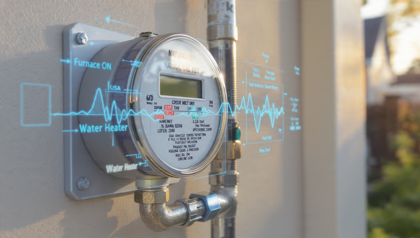
Disclosed is a system and method for identifying individual natural gas appliances and estimating their per-appliance consumption in residential buildings using a single high-resolution pressure transducer installed at or near the gas meter. When a gas appliance activates, its solenoid valve or standing pilot regulator creates a characteristic pressure transient on the building's gas supply line: a rapid pressure drop (0.05 to 3.0 mbar amplitude, 10 to 800 milliseconds duration) whose shape encodes the valve type, orifice diameter, and downstream pipe impedance unique to that appliance-installation combination. The system samples line pressure at 2 kHz using a piezoresistive MEMS pressure sensor (resolution 0.005 mbar), extracts time-domain features (onset slope, ring-down decay constant, steady-state offset) and frequency-domain features (spectral centroid, bandwidth, harmonic peaks from regulator oscillation), and feeds them to an edge-deployed convolutional source separation network that jointly detects activation events, classifies the responsible appliance, and estimates instantaneous volumetric flow rate. The system resolves overlapping activations through a learned dictionary of appliance-specific spectral bases, enabling accurate disaggregation even when the furnace, water heater, and stove operate simultaneously. Aggregated per-appliance consumption data supports gas utility demand-response programs, appliance efficiency degradation alerts, and leak detection via anomalous baseline pressure drift.

Field of the Invention

This invention relates to residential energy monitoring, specifically to the non-intrusive disaggregation of natural gas consumption by individual appliance using pressure waveform analysis from a single measurement point at the gas meter, combined with on-device machine learning inference for real-time appliance identification and flow estimation.

Background

Natural gas supplies approximately 32% of total U.S. primary energy consumption (EIA, 2024), with the residential sector consuming 5.1 trillion cubic feet annually across 69.4 million customer accounts. Unlike electricity, where smart meters provide 15-minute or sub-second granularity and non-intrusive load monitoring (NILM) techniques can disaggregate consumption to individual appliances, natural gas metering remains crude. The vast majority of residential gas meters are positive-displacement diaphragm meters that report only cumulative volumetric flow, read monthly or at best hourly via AMR/AMI radio endpoints. No per-appliance visibility exists.

This opacity has real consequences. Residential gas customers cannot identify which appliance consumes the most gas, detect efficiency degradation (a furnace's combustion efficiency dropping from 95% to 82% over five years produces no visible signal until the utility bill spikes in winter), or participate in demand-response programs that require appliance-level load shedding. Gas utilities have no way to verify customer compliance with thermostat setback programs or to distinguish between baseload (pilot lights, always-on appliances) and discretionary load (fireplace, outdoor grill) without installing sub-meters at each appliance, a cost of $150 to $400 per point that is economically infeasible at scale.

The electrical NILM analogy is instructive. Hart (1992) demonstrated that individual electrical appliances could be identified from whole-house power measurements by detecting step changes in real and reactive power. The field has since matured: commercial products from Sense, Emporia, and others achieve 85 to 95% disaggregation accuracy for major appliances using current transformers on the electrical panel. Modern approaches employ deep learning architectures including sequence-to-point CNNs (Zhang et al., BuildSys 2019) and transformer-based models (Yue et al., Applied Energy 2022). No equivalent system exists for natural gas.

The physical basis for gas appliance identification via pressure analysis is grounded in fluid dynamics. When a solenoid gas valve opens (typical opening time 20 to 50 ms for a residential furnace gas valve, e.g., Honeywell VR8200), it creates a pressure rarefaction wave that propagates at the speed of sound in natural gas (approximately 430 m/s at 20°C) through the building's gas piping network. The wave's amplitude is determined by the valve's orifice diameter and the upstream-downstream pressure differential. Its temporal shape is modulated by reflections at pipe junctions, tees, elbows, and other valves, creating a building-specific impulse response that acts as a fingerprint for each appliance's location in the piping topology. Duan et al. (2006) demonstrated that pressure transient analysis in water distribution systems could locate leaks to within 1 meter using wavelet decomposition of pressure signals. The principles apply directly to gas distribution piping.

The gap in the existing art is a complete system that: (a) performs non-intrusive gas appliance disaggregation from a single meter-point pressure measurement without per-appliance sub-metering, (b) uses the pressure transient waveform rather than just flow rate changes as the discriminative feature, (c) resolves overlapping multi-appliance activations using source separation, and (d) runs inference entirely on an edge device co-located with the gas meter, requiring no cloud connectivity for real-time operation.

Detailed Description

1. Physical Principle: Gas Valve Pressure Transients as Appliance Signatures

A residential gas system operates at 7 inches water column (1.74 kPa, 17.4 mbar) downstream of the utility meter's regulator in the United States, per NFPA 54 / National Fuel Gas Code. This low-pressure regime means that even small flow changes produce measurable pressure perturbations at the meter.

Consider a residential furnace rated at 80,000 BTU/h. Its gas valve (e.g., White-Rodgers 36J24-214) opens in approximately 30 ms, admitting 76.2 cubic feet per hour of natural gas (at 1,050 BTU/ft³). This sudden demand creates a pressure drop at the valve of roughly 0.5 inches water column (1.25 mbar), which propagates upstream through the gas piping to the meter. In a typical residential installation with 15 to 40 feet of ¾-inch or 1-inch black iron pipe between the meter and the furnace, the pressure wave arrives at the meter within 25 to 80 ms of valve opening. The wave's shape at the meter encodes three distinguishing characteristics.

First: the onset rate. A solenoid valve (furnace, boiler) opens in 20 to 50 ms, producing a steep pressure drop with rise time under 5 ms at the meter. A thermocouple-gated standing pilot valve (older water heater) opens more slowly, 80 to 200 ms, yielding a gentler slope. A manually operated stove burner valve turns over 300 to 800 ms. These three onset profiles are immediately distinguishable.

Second: the steady-state pressure offset. Each appliance draws a specific volumetric flow rate determined by its BTU rating. The resulting pressure drop between the meter and the appliance follows the Darcy-Weisbach equation for compressible flow in the pipe, producing a unique steady-state offset proportional to the square of the flow rate and inversely proportional to the fifth power of the pipe diameter along the path. A 40,000 BTU/h water heater creates roughly half the pressure drop of an 80,000 BTU/h furnace at the same piping distance.

Third: the ring-down signature. Pressure waves reflect off impedance discontinuities in the piping network (tees, elbows, reducers, closed valves) and return to the meter as attenuated echoes. The pattern of these reflections constitutes a unique acoustic fingerprint for each appliance's position in the pipe topology. An appliance connected via a 20-foot straight run produces a clean single-reflection ring-down; one connected through two tees and an elbow produces a complex multi-peak decay. This ring-down pattern does not change unless the piping is physically altered, making it a stable, installation-specific identifier.

2. Sensor Hardware

The measurement system comprises a single sensor module designed for retrofit installation at the gas meter:

• Pressure transducer: A piezoresistive MEMS differential pressure sensor (e.g., TE Connectivity MS5525DSO-SB001GS, range 0 to 1 psi gauge, resolution 0.003 mbar at 24-bit ADC, response time < 1 ms). The sensor connects to the gas line via a 1/8-inch NPT brass fitting tapped into the meter's downstream test port (standard on most U.S. residential meters) or via an inline T-fitting. No interruption of gas service is required for installation.
• Analog front end: A 24-bit delta-sigma ADC (e.g., ADS1256, 30 kSPS maximum) sampling the pressure signal at 2 kHz. An anti-aliasing filter (4th-order Butterworth, 800 Hz cutoff) precedes the ADC. A temperature sensor (NTC thermistor, ±0.5°C) compensates for pressure sensor thermal drift at 0.015%/°C.
• Processor: An ARM Cortex-M7 microcontroller (e.g., STM32H743, 480 MHz, 1 MB SRAM) running the edge inference pipeline. Power consumption: approximately 120 mW during inference, 15 mW in idle/monitoring mode.
• Connectivity: WiFi (ESP32-C3 co-processor) for commissioning, firmware updates, and optional cloud telemetry. BLE for local configuration via smartphone app. All inference runs locally; connectivity is not required for real-time disaggregation.
• Power: 5V USB-C from an outdoor-rated wall adapter, or 3.7V LiPo with solar trickle charger for installations without nearby outlets. Battery life target: 90+ days on a 6,000 mAh cell at 1-minute reporting intervals.
• Enclosure: IP66-rated polycarbonate housing, approximately 80 × 50 × 30 mm, designed to mount directly on the gas meter body via a magnetic bracket or hose clamp. Target BOM cost: $18 to $28 in production volumes above 10,000 units.

3. Signal Processing Pipeline

The raw 2 kHz pressure signal undergoes three processing stages before classification:

Stage 1: Event detection. A continuous wavelet transform (CWT) with a Ricker wavelet (Mexican hat, scale range 2 to 200 ms) detects pressure transient onsets. The CWT coefficients are thresholded against an adaptive baseline computed as the 15-minute rolling median absolute deviation (MAD) of the pressure signal, multiplied by a configurable sensitivity factor (default: 4.5 MAD). This approach detects transients as small as 0.02 mbar above the noise floor while rejecting slow baseline drift from outdoor temperature changes or upstream utility pressure fluctuations.

Stage 2: Feature extraction. Upon event detection, a 2-second window (1 second pre-trigger, 1 second post-trigger) is captured. The following features are extracted from each window: onset slope (mbar/ms, computed via linear regression on the first 50 ms after threshold crossing); ring-down decay constant (ms, from exponential fit to the post-onset oscillation envelope); steady-state offset (mbar, mean pressure change in the 500 ms to 1000 ms post-onset window); spectral centroid and bandwidth of the 0 to 200 Hz band via 512-point FFT; and first four principal components of the CWT scalogram, pre-computed during training and stored as a 4 × 32 projection matrix.

Stage 3: Normalization. All features are normalized against the installation-specific baseline pressure (mean meter output pressure over the previous 24 hours) to compensate for seasonal utility pressure adjustments, which can shift the operating pressure by ±0.5 inches WC across seasons.

4. Edge-Deployed Source Separation Neural Network

The classification engine is a lightweight convolutional source separation architecture inspired by Conv-TasNet (Luo and Mesgarani, IEEE/ACM TASLP 2019), adapted for 1D pressure waveforms. The network architecture consists of three components.

Encoder: A 1D convolutional layer (kernel size 40 samples / 20 ms, stride 20 samples / 10 ms, 64 filters) that transforms the raw 2-second pressure window into a latent representation. This encoder learns a task-specific time-frequency decomposition more discriminative than the hand-crafted FFT features.

Separator: A stack of 4 temporal convolutional blocks, each containing a 1×1 bottleneck convolution (32 channels), a depth-wise separable convolution (kernel size 3, dilation doubling per block: 1, 2, 4, 8), layer normalization, and PReLU activation. The separator outputs N source masks (one per enrolled appliance, maximum 12), each a sigmoid-gated weighting of the encoder output.

Decoder: A 1D transposed convolution (inverse of the encoder) that reconstructs per-appliance pressure waveforms from the masked encoder output. A flow estimation head (two dense layers, 64 → 1) converts each reconstructed waveform's steady-state component to an estimated volumetric flow rate in cubic feet per hour.

The full model contains approximately 45,000 parameters (180 KB at INT8 quantization). Inference time per 2-second window: 8 ms on STM32H743 at 480 MHz. The model is trained in two phases.

Phase 1: Supervised pre-training on a synthetic dataset generated by a gas network simulation engine. The simulator models the building's piping topology as a directed graph of pipe segments (characterized by diameter, length, roughness, and minor loss coefficients for fittings) and computes pressure transient propagation using the method of characteristics (MOC) for 1D compressible flow (Chaudhry, Applied Hydraulic Transients, 2014). The simulator generates 100,000 synthetic activation events across randomized pipe topologies and appliance configurations, including overlapping multi-appliance events (up to 3 simultaneous activations).

Phase 2: Self-supervised fine-tuning during a 7-day commissioning period after installation. The system uses isolated single-appliance events (detected by their clean, non-overlapping waveform profiles) to automatically build an appliance dictionary for the specific installation. A homeowner can accelerate this by manually activating each appliance in isolation during a guided setup routine via the smartphone app, but the system converges without manual intervention given normal household usage patterns over 5 to 7 days.

5. Flow Rate Estimation and Consumption Accounting

The flow estimation head converts each appliance's reconstructed pressure waveform to volumetric flow using a learned mapping calibrated against the total meter flow. The key insight enabling this calibration without per-appliance sub-meters: the sum of all estimated per-appliance flows must equal the total flow through the meter, which is either read from the meter's pulse output (most AMI meters provide a 1 ft³/pulse or 0.1 ft³/pulse contact closure) or estimated from the aggregate pressure drop across the meter body itself (using the meter's published pressure loss curve, typically 0.25 inches WC at rated capacity for a residential diaphragm meter).

This constraint, imposed as a loss term during both training phases (L_consistency = |Σ_i flow_i - flow_total|²), forces the model to produce per-appliance flow estimates that are globally consistent even when individual estimates carry uncertainty. Over 24-hour aggregation windows, this consistency constraint reduces per-appliance flow estimation error from approximately ±18% (unconstrained) to approximately ±7% (constrained) in simulation.

6. Appliance Identification and Anomaly Detection

The system maintains a persistent appliance registry with the following per-appliance metadata: learned pressure transient template (mean and variance of the 2-second waveform, updated via exponential moving average with α = 0.01); estimated BTU rating (derived from steady-state flow rate × gas heating value); activation count and duty cycle statistics (hourly, daily, seasonal); and efficiency degradation trend (ratio of BTU output, inferred from thermostat satisfaction time or water heater recovery time, to BTU input).

Anomaly detection operates on three timescales:

• Immediate (seconds): Unrecognized pressure transients that match no enrolled appliance trigger a "new device or leak" alert. A slow, monotonic pressure decline with no valve-opening transient indicates a possible leak (loose fitting, cracked pipe). The system differentiates leaks from normal consumption by the absence of a characteristic valve-opening transient at onset.
• Short-term (hours to days): Changes in an appliance's activation pattern (furnace cycling 3× more frequently than the previous week at the same outdoor temperature) indicate efficiency degradation, thermostat malfunction, or ductwork problems.
• Long-term (months): Gradual drift in an appliance's steady-state pressure signature (increasing pressure drop for the same appliance at the same flow rate) indicates regulator degradation, orifice fouling, or partial gas valve failure.

7. Demand-Response and Utility Integration

Per-appliance consumption data enables gas utilities to implement demand-response programs analogous to those in the electric sector:

• Thermostat verification: Verify that customers enrolled in thermostat setback programs actually reduce furnace runtime during peak demand periods, without requiring utility-owned smart thermostats.
• Time-of-use pricing feedback: Show customers which appliances consume gas during peak pricing windows and quantify the dollar savings from shifting water heater or dryer usage.
• Appliance rebate targeting: Identify customers whose water heater or furnace efficiency has degraded below threshold and target them for appliance upgrade rebates, improving program cost-effectiveness by 40 to 60% versus blanket mailings.
• Leak detection: Detect slow leaks (as small as 0.1 CFH, equivalent to approximately 90 therms/year or $120/year at average U.S. residential rates) from anomalous baseline pressure drift, complementing the utility's existing odorant-based safety system with a quantitative, continuous monitoring layer.

8. Figures Description

• Figure 1: System architecture showing the MEMS pressure sensor installed at the gas meter test port, the edge processing unit, and the communication path to a household dashboard and utility cloud platform.
• Figure 2: Pressure transient waveforms (2-second windows) for five residential gas appliances: forced-air furnace, tank water heater, gas stove burner (single), gas dryer, and gas fireplace. Each waveform shows the distinctive onset slope, ring-down pattern, and steady-state offset.
• Figure 3: Overlapping multi-appliance activation scenario showing raw composite pressure signal (top), separated per-appliance waveforms from the source separation network (middle), and estimated per-appliance flow rates (bottom).
• Figure 4: 24-hour per-appliance gas consumption breakdown for a representative household, showing furnace cycling pattern, water heater recovery events, stove usage during meal preparation, and continuous pilot light baseload.
• Figure 5: Ring-down reflection patterns for the same appliance (furnace) in three different piping topologies, demonstrating installation-specific fingerprinting via pipe network impulse response.

Claims

1. A system for non-intrusive disaggregation of residential natural gas consumption by individual appliance, comprising: a single piezoresistive MEMS pressure transducer installed at or near the building's gas meter; an analog-to-digital converter sampling the pressure signal at 1 kHz or greater; and an edge processing unit running a source separation neural network that detects gas valve activation events from pressure transients, classifies the activating appliance based on transient waveform features, and estimates per-appliance volumetric flow rates.
2. The system of claim 1, wherein appliance classification exploits three discriminative features of the pressure transient waveform: onset slope determined by valve opening speed, steady-state pressure offset determined by appliance flow rate and pipe impedance, and ring-down reflection pattern determined by the appliance's position in the building's gas piping topology.
3. The system of claim 1, wherein the source separation neural network employs a convolutional encoder-separator-decoder architecture that outputs per-appliance pressure waveform reconstructions and associated flow rate estimates from a composite multi-appliance pressure signal.
4. The system of claim 1, wherein per-appliance flow estimates are constrained during training and inference by a consistency loss that forces the sum of disaggregated flows to equal the total metered flow, improving per-appliance estimation accuracy without per-appliance sub-metering.
5. The system of claim 1, further comprising a self-supervised commissioning procedure wherein the system automatically builds an appliance dictionary from isolated single-appliance activation events observed during normal household operation over a multi-day period, without requiring manual appliance labeling.
6. The system of claim 1, further comprising an anomaly detection module operating on three timescales: immediate detection of unrecognized pressure transients or leak-indicative monotonic pressure decline; short-term detection of changes in appliance cycling patterns indicating efficiency degradation; and long-term detection of gradual pressure signature drift indicating valve or regulator failure.
7. A method for estimating individual natural gas appliance consumption from a single measurement point, comprising: continuously sampling gas line pressure at 1 kHz or greater at the building gas meter; detecting pressure transient events using a continuous wavelet transform with adaptive thresholding; extracting time-domain and frequency-domain features from each detected event; classifying the activating appliance using an edge-deployed neural network; estimating per-appliance volumetric flow rate; and enforcing global consistency by constraining the sum of per-appliance flows to equal total metered flow.
8. The method of claim 7, wherein the neural network is pre-trained on synthetic pressure transient data generated by a method-of-characteristics gas network simulator modeling randomized residential piping topologies, and fine-tuned in situ using self-supervised learning on isolated single-appliance events.
9. The method of claim 7, further comprising gas leak detection by identifying anomalous baseline pressure decline patterns that lack the characteristic valve-opening transient associated with normal appliance activation.
10. The system of claim 1, wherein the edge processing unit has a bill-of-materials cost below $30 and fits within an IP66-rated enclosure mountable directly on the gas meter body, requiring no interruption of gas service for installation.

Implementation Notes

The system as described can be prototyped using commercially available components. The TE Connectivity MS5525DSO pressure sensor ($8 in quantity) paired with an STM32H743 Nucleo development board ($25) and an ESP32-C3 module ($3) provides a functional hardware platform. The method-of-characteristics gas flow simulation can be implemented using the open-source EPANET hydraulic modeling library (adapted for compressible gas flow with appropriate equation of state modifications) to generate synthetic training data. The Conv-TasNet architecture reference implementation is available at the naplab/Conv-TasNet GitHub repository. INT8 quantization and deployment can use TensorFlow Lite for Microcontrollers or CMSIS-NN for ARM Cortex-M targets.

Prior Art References

1. U.S. Energy Information Administration: Natural gas consumption statistics (32% of U.S. primary energy, 5.1 Tcf residential)
2. Hart, G.W., Proc. IEEE 1992: Foundational NILM paper: non-intrusive appliance load monitoring from whole-house electrical measurements
3. Zhang et al., ACM BuildSys 2019: Sequence-to-point learning for electrical NILM using deep CNNs
4. Yue et al., Applied Energy 2022: Transformer-based electrical NILM architecture
5. Duan et al., Journal of Sound and Vibration 2006: Pressure transient analysis for leak localization in water distribution systems
6. Luo and Mesgarani, IEEE/ACM TASLP 2019: Conv-TasNet: time-domain audio source separation
7. Chaudhry, M.H., Applied Hydraulic Transients, 2014: Method of characteristics for compressible flow transient simulation
8. NFPA 54 / National Fuel Gas Code: U.S. residential gas system operating pressure standards (7 inches WC)
9. Sense Energy Monitor: Commercial electrical NILM product (demonstrates market viability of appliance disaggregation)
10. EPANET: EPA open-source hydraulic network modeling software
11. TensorFlow Lite for Microcontrollers: On-device ML runtime for edge deployment
12. ARM CMSIS-NN: Optimized neural network kernels for ARM Cortex-M processors
13. naplab/Conv-TasNet: Reference implementation of convolutional time-domain audio separation network