System and Method for Real-Time Urban Three-Dimensional Wind Field Reconstruction Using Flight Controller Correction Telemetry from Commercial Delivery Drone Fleets with Graph Neural Network Spatiotemporal Interpolation

Abstract

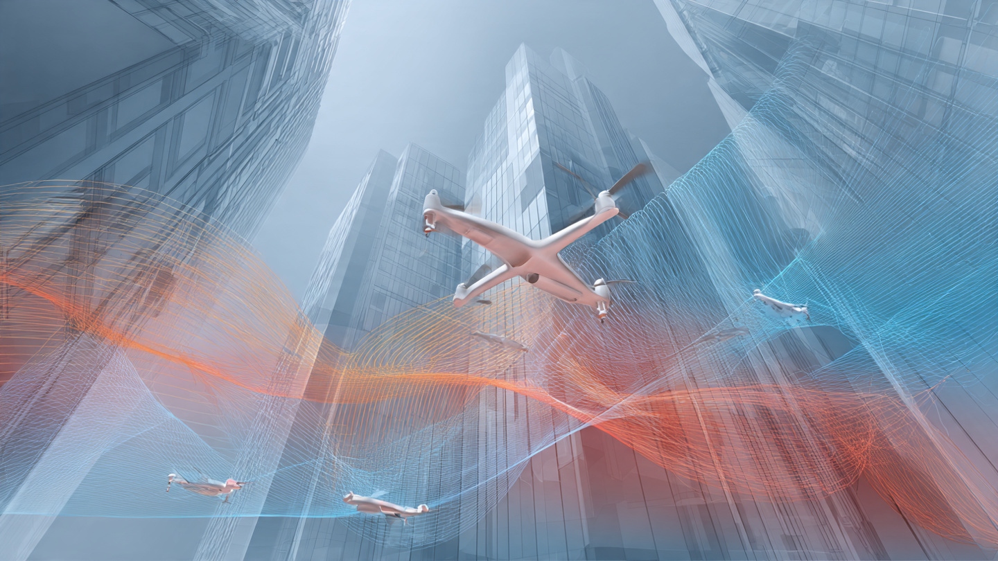
Disclosed is a system and method for continuously reconstructing three-dimensional wind velocity fields over urban areas by analyzing flight controller correction telemetry from commercial delivery drone fleets. Each multirotor drone's autopilot continuously adjusts motor RPMs to maintain its planned trajectory against aerodynamic disturbances. The difference between the commanded attitude/thrust vector and the corrections applied by the PID (proportional-integral-derivative) control loop encodes the instantaneous wind velocity vector experienced by that aircraft at its GPS-reported position and altitude. A lightweight edge inference module (12,000 parameters, 24 KB INT8) running on the drone's existing flight controller extracts wind speed estimates (horizontal and vertical components) at 2 Hz from the control correction signal, motor current telemetry, and IMU data, transmitting only a 48-byte wind observation packet per sample via the drone's existing cellular data link. A cloud-hosted graph neural network (340,000 parameters) with dynamic graph construction treats each drone observation as a spatiotemporal node, builds edges based on proximity and building geometry from a 3D city model, and interpolates the sparse, mobile observations into a continuous volumetric wind field at 25-meter horizontal and 10-meter vertical resolution, updated every 30 seconds. The system requires no additional sensors on the drones, no dedicated weather infrastructure, and produces wind field reconstructions across altitude bands from 15 to 120 meters AGL that conventional surface weather stations and mesoscale models cannot resolve.

Field of the Invention

This invention relates to atmospheric sensing and urban meteorology, specifically to methods for reconstructing spatially continuous three-dimensional wind fields using opportunistic telemetry from commercial unmanned aerial vehicle fleets and machine learning interpolation.

Background

Urban wind fields are among the least observed and most complex atmospheric phenomena. Buildings create channeling effects, vortex shedding, downwash, and turbulent wakes that vary on scales of meters and seconds. These wind patterns directly affect pedestrian comfort, pollutant dispersion, wildfire smoke transport, building energy loads, and the safety of urban air mobility (UAM) operations. Yet the observational infrastructure available to characterize them is sparse and surface-bound.

Current urban wind observation methods suffer from fundamental coverage limitations:

• Surface weather stations: The Automated Surface Observing System (ASOS) network provides measurements at approximately 900 US airports at 10-meter height. Station spacing in urban areas is typically 10-50 km. These stations measure wind at a single altitude, far from building-influenced zones, and cannot resolve street-level or rooftop-level flows. Muller et al. (2013) demonstrated that urban surface stations systematically underestimate peak winds by 30-50% compared to above-canopy measurements.
• Sonic anemometer arrays: Research-grade 3D sonic anemometers (e.g., Campbell Scientific CSAT3B, $4,500/unit) provide 20 Hz, three-component wind measurements at a single point. Urban field campaigns such as DAPPLE (London, 2003-2004) and JOINT URBAN 2003 (Oklahoma City) deployed dense arrays of 30-100 anemometers but cost $500,000-$2M, ran for weeks to months, and covered areas smaller than 1 km². No city maintains permanent dense anemometer coverage.
• Doppler lidar: Scanning Doppler wind lidars can profile wind at ranges up to 10 km with 50-meter range gates. Units cost $150,000-$500,000 each. A single lidar provides line-of-sight velocity along its beam direction; full 3D wind reconstruction requires three or more units in a Dual-Doppler or Triple-Doppler configuration, impractical for city-wide coverage.
• Computational Fluid Dynamics (CFD): Steady-state Reynolds-Averaged Navier-Stokes (RANS) simulations of urban wind require 3D building geometry, boundary conditions from mesoscale models, and hours to days of compute time per scenario. Large Eddy Simulation (LES) provides time-resolved results but requires supercomputer resources. Neither approach provides real-time observations; both are simulations conditioned on sparse boundary data.
• Mesoscale numerical weather prediction: Models like WRF operate at 1-3 km horizontal resolution in their finest nests, far too coarse to resolve individual building wakes. The HRRR model provides 3 km resolution hourly updates but treats urban areas as bulk roughness elements, not resolved geometry.

Meanwhile, commercial delivery drone fleets are scaling rapidly. Wing (Alphabet) surpassed 350,000 deliveries by early 2024 and operates in multiple US metro areas. Amazon Prime Air launched in multiple cities in 2024-2025. Zipline operates in seven countries with its P2 platform for instant delivery. Each of these fleets fields hundreds of drones making thousands of daily flights across urban and suburban areas at altitudes of 30-120 meters AGL, precisely the altitude band that conventional observations cannot reach. Every one of these drones carries a flight controller with an IMU (accelerometer and gyroscope), GPS receiver, barometric altimeter, and motor speed controllers, and every flight controller continuously computes control corrections that encode the wind environment the drone is traversing.

Prior work has demonstrated the feasibility of wind estimation from multirotor telemetry. Palomaki et al. (Sensors, 2017) estimated wind speed and direction from a quadrotor's attitude angles and motor RPMs with RMSE of 0.5 m/s against a collocated sonic anemometer. Barbieri et al. (Meteorological Applications, 2019) used DJI Phantom data to profile wind in the atmospheric boundary layer. Thielicke et al. (AMT, 2021) demonstrated wind estimation accuracy of ±0.3 m/s from a custom hexacopter in controlled conditions. However, all prior work treats drones as isolated meteorological instruments. No system has been disclosed that: (a) extracts wind estimates from fleet-scale commercial delivery operations without additional sensors; (b) uses graph neural networks to interpolate between the mobile, sparse, irregularly-spaced observations; (c) incorporates 3D building geometry as prior knowledge in the interpolation; or (d) produces a continuous volumetric wind field product updated in near-real-time.

Detailed Description

1. Wind Estimation from Flight Controller Corrections

A multirotor drone in steady-state horizontal flight maintains equilibrium between gravity, thrust, drag, and the aerodynamic force from wind. The flight controller's PID loop commands motor RPMs to achieve the attitude (roll φ, pitch θ, yaw ψ) and thrust magnitude needed to follow the planned trajectory. When a wind gust displaces the drone, the controller responds with corrective commands. The difference between the trim condition (the attitude/thrust that would be required in still air for the current trajectory) and the actual commanded values encodes the wind disturbance.

For a quadrotor of mass m in horizontal flight through a wind field with horizontal components (Wx, Wy) and vertical component Wz:

The horizontal wind components relate to the drone's tilt angles by: Wx ≈ (m × g × tan(θ_correction)) / (0.5 × ρ × Cd × A), where θ_correction is the pitch angle deviation from the zero-wind trim, ρ is air density (~1.15 kg/m³ at typical delivery altitudes), Cd is the drone's drag coefficient (~1.0-1.3 for multirotor frames), and A is the effective frontal area (~0.03-0.08 m² for delivery-class drones). An analogous expression governs the roll axis for Wy.

The vertical wind component Wz is estimated from the thrust deviation: Wz ≈ (T_actual - T_trim) / (0.5 × ρ × Cd_z × A_z), where T_actual is the total thrust computed from measured motor RPMs and known motor thrust coefficients (KT), and T_trim is the thrust required for steady flight in still air (approximately m × g / cos(total_tilt)).

Motor RPMs are obtained either from electronic speed controller (ESC) telemetry (available on most commercial flight controllers via DShot or BLHeli protocols) or inferred from motor current measurements using the known motor velocity constant (KV). The motor thrust coefficient KT is calibrated per drone model using static thrust stand data, with in-flight refinement using periods of GPS-verified zero-wind conditions (calm dawn flights, sheltered corridors between buildings).

2. Edge Inference Module

A lightweight wind estimation model runs on the drone's existing flight controller processor (typically STM32H7-class, ARM Cortex-M7 at 480 MHz with FPU). The model processes a 50-element input vector at 2 Hz containing: PID correction outputs for roll, pitch, yaw, and thrust (8 values: P, I, D terms for attitude plus thrust correction); motor RPM or current for each motor (4-8 values depending on configuration); IMU readings (accelerometer 3-axis, gyroscope 3-axis); GPS velocity (3-axis, from the navigation filter); barometric altitude and temperature; and airspeed estimate from the extended Kalman filter (if available). The model architecture is a 3-layer fully connected network (50 → 32 → 16 → 3, ReLU activations) with residual connections, totaling 12,000 parameters (24 KB quantized to INT8). Inference time is under 0.5 ms per sample on Cortex-M7. The model outputs a 3D wind velocity vector (Wx, Wy, Wz) in the local North-East-Down frame.

Training data is generated from paired flights: drones carrying calibrated sonic anemometers (truth data) fly alongside or in formation with standard delivery drones. A dataset of 10,000+ flight hours across diverse urban environments, wind conditions (0-15 m/s), and drone payloads (0-2.5 kg) provides the supervised learning signal. Data augmentation includes synthetic wind fields from LES simulations applied to drone dynamics models.

The model is calibrated per drone model and payload weight class. Payload mass affects the trim thrust and attitude, so the model accepts a payload weight input (known from the delivery manifest) as a conditioning variable. Target accuracy: ±0.8 m/s horizontal, ±0.5 m/s vertical for winds up to 12 m/s.

3. Observation Packet Transmission

Each wind observation is encoded as a 48-byte packet: latitude (4 bytes, fixed-point 1e-7 degrees), longitude (4 bytes), altitude AGL (2 bytes, 0.1 m resolution), timestamp (4 bytes, Unix epoch seconds), Wx (2 bytes, signed, 0.01 m/s resolution), Wy (2 bytes), Wz (2 bytes), wind speed uncertainty estimate (2 bytes), drone model ID (2 bytes), payload weight class (1 byte), flight phase flag (1 byte: cruise/ascend/descend/hover), and a 22-byte reserved/checksum field. Packets are transmitted via the drone's existing LTE or 5G cellular data link as UDP datagrams to the aggregation server, piggy-backing on the telemetry channel already used for fleet management. At 2 Hz sampling, each drone generates 96 bytes/second of wind data, negligible compared to the video/telemetry bandwidth already consumed.

4. Graph Neural Network Spatiotemporal Interpolation

The core interpolation engine is a spatiotemporal graph neural network that constructs a dynamic graph from incoming drone observations and outputs a continuous volumetric wind field. The architecture operates in three stages:

Stage 1: Dynamic graph construction. Each wind observation within a sliding 5-minute temporal window becomes a node in the graph. Node features include the 3D position, timestamp, wind vector estimate, uncertainty, flight phase, and altitude class. Edges are constructed between nodes using three criteria: (a) spatial proximity (nodes within 200 m horizontal, 30 m vertical); (b) line-of-sight connectivity (edges are suppressed between nodes separated by buildings, using a ray-casting test against a 3D building geometry model from Cesium 3D Tiles or OpenStreetMap LOD2 building data); and (c) fluid dynamical adjacency (edges are added between nodes that are upstream/downstream of each other based on the estimated mean flow direction, even if they are farther than the proximity threshold, to capture advection). Edge features encode the 3D displacement vector, the building obstruction flag, and the time offset between observations.

Stage 2: Message-passing layers. Four graph attention network (GAT) layers with 64 hidden dimensions per head and 4 attention heads process the graph. Each layer applies multi-head attention where the attention weights learn to prioritize observations that are aerodynamically relevant (e.g., an observation in a building wake attends strongly to the upstream observation above the roofline rather than a laterally adjacent observation behind a different building). The attention mechanism incorporates the edge features, so building geometry directly modulates information flow. Residual connections and layer normalization are applied after each GAT layer.

Stage 3: Volumetric field decode. The output is a continuous wind field sampled at query points on a regular 3D grid (25 m horizontal, 10 m vertical resolution) covering the urban area of interest. Each query point attends to the k=16 nearest graph nodes via a cross-attention mechanism, producing a wind velocity vector and uncertainty estimate at every grid point. The decoder includes a physics-informed loss term that penalizes solutions violating the incompressible continuity equation (∇·u = 0, appropriate for low Mach number urban flows) and boundary conditions (zero normal velocity at building surfaces). Total model parameters: 340,000 (680 KB FP16). Inference time for a 5 km × 5 km × 0.1 km volume: approximately 2 seconds on a single NVIDIA T4 GPU.

5. 3D Building Geometry Integration

The system ingests 3D building models from municipal GIS databases, OpenStreetMap with height attributes, or commercial providers (Cesium, Google 3D Tiles). Building geometry serves three roles in the pipeline: (a) graph edge suppression by blocking line-of-sight connections between observations separated by solid structures; (b) boundary condition enforcement at building surfaces in the physics-informed loss; and (c) prior knowledge injection via a building-wake parameterization module that provides initial wind field estimates in the lee of buildings based on the ESDU 85038 wake model, conditioned on the upstream wind speed and building aspect ratio. This parameterization fills in wind estimates in regions where no drone observations are available (e.g., narrow alleys or courtyards that delivery drones do not traverse).

6. Calibration and Validation

The system maintains continuous self-calibration through three mechanisms: (a) inter-drone consistency checks, where two drones passing within 50 m and 30 seconds of each other should report similar wind vectors, and systematic discrepancies trigger per-drone bias corrections; (b) surface station anchoring, where wind observations from drones transiting near ASOS or mesonet stations are compared against the station readings (adjusted for altitude using a logarithmic wind profile), providing an absolute reference; and (c) GPS ground speed residuals, where the difference between GPS-measured ground speed and the drone's estimated airspeed provides an independent wind speed estimate that cross-checks the controller-based method.

7. Applications

• Urban air mobility (UAM) corridor planning: Identify persistent high-turbulence zones, channeling corridors, and calm-air paths for eVTOL approach/departure routing. Update turbulence advisories in real-time for vertiport operations. FAA UAM ConOps identifies wind hazard assessment as a critical gap.
• Pedestrian wind comfort: City planners and architects currently rely on wind tunnel tests or CFD simulations for pedestrian wind comfort assessments (Lawson criterion). The system provides continuous real-world validation data at rooftop and street-canyon scales for proposed and existing developments.
• Pollutant and wildfire smoke dispersion: Feeding observed 3D wind fields into atmospheric dispersion models (e.g., AERMOD, ALOHA) replaces assumed wind profiles with measured fields, improving pollutant concentration predictions in urban canyons where channeling can increase street-level concentrations by 2-5x relative to open-terrain estimates.
• Building energy modeling: Convective heat transfer coefficients on building facades depend on local wind speed. The volumetric wind field enables facade-resolved wind speed inputs for building energy simulation tools (EnergyPlus), improving HVAC load predictions by an estimated 8-15% for tall buildings in dense urban cores.
• Mesoscale model assimilation: The wind observations at 15-120 m AGL fill a critical gap in the atmospheric observing system. Assimilating drone-derived wind profiles into the HRRR or WRF models via 3D-Var or ensemble Kalman filter methods could improve urban boundary layer forecasts, particularly for the low-level jet and nocturnal wind transitions that surface stations miss.

8. Figures Description

• Figure 1: System architecture showing delivery drone fleet generating wind observations during normal operations, cellular uplink of observation packets, graph neural network interpolation engine, and output wind field products.
• Figure 2: Schematic of wind estimation from flight controller corrections, showing the relationship between PID output, motor RPM adjustments, drone tilt angles, and the inferred wind vector.
• Figure 3: Dynamic graph construction over a 5-minute window in a 2 km × 2 km urban area, with drone trajectory observations as nodes, proximity and line-of-sight edges, and building geometry suppressing edges through solid structures.
• Figure 4: Example reconstructed 3D wind field cross-section through a downtown canyon, showing accelerated flow above roofline, deceleration in the wake zone, and channeling at street level, with drone observation positions marked.

Claims

1. A system for reconstructing three-dimensional urban wind fields, comprising: a fleet of commercial delivery drones, each equipped with a flight controller having an inertial measurement unit, GPS receiver, and motor speed controllers; an edge inference module running on each drone's flight controller that extracts wind velocity vector estimates from the flight controller's PID correction outputs, motor telemetry, and IMU data without additional meteorological sensors; and a cloud-hosted graph neural network that receives wind observations from multiple drones and interpolates them into a continuous volumetric wind field over an urban area.
2. The system of claim 1, wherein the edge inference module estimates wind velocity by computing the difference between the drone's trim attitude and thrust (the values required for the current trajectory in still air) and the actual attitude and thrust corrections commanded by the PID control loop, relating the correction magnitude to wind speed through calibrated aerodynamic drag and thrust coefficients.
3. The system of claim 1, wherein the graph neural network constructs a dynamic graph from drone observations within a sliding temporal window, with edges between nodes determined by spatial proximity, temporal proximity, and line-of-sight connectivity tested against a three-dimensional building geometry model.
4. The system of claim 3, wherein the graph neural network suppresses edges between observation nodes that are separated by solid building structures using ray-casting against a 3D city model, preventing non-physical information flow across building barriers.
5. The system of claim 1, wherein the graph neural network incorporates a physics-informed loss term that penalizes wind field solutions violating the incompressible continuity equation and enforces zero normal velocity boundary conditions at building surfaces.
6. The system of claim 1, wherein each drone transmits wind observation packets of 48 bytes or fewer at a rate of 1-10 Hz via its existing cellular data link, the packets comprising position, altitude, timestamp, three-component wind vector, uncertainty estimate, and drone configuration metadata.
7. A method for urban atmospheric sensing comprising: operating a fleet of commercial delivery drones along planned delivery routes through an urban area; extracting, on each drone's flight controller, a three-component wind velocity estimate from the controller's PID correction signals and motor telemetry at a rate of at least 1 Hz during flight; transmitting the wind estimates along with position and timestamp metadata to an aggregation service; constructing a spatiotemporal graph from the aggregated observations; processing the graph through a graph attention network that interpolates between observations while respecting building geometry constraints; and producing a gridded three-dimensional wind field at a spatial resolution finer than 50 meters horizontal and 20 meters vertical, updated at intervals shorter than 5 minutes.
8. The method of claim 7, further comprising a self-calibration mechanism that compares wind estimates from two or more drones transiting within a specified spatial and temporal proximity, computing per-drone bias corrections when systematic discrepancies exceed a threshold.
9. The method of claim 7, further comprising anchoring the drone-derived wind observations against surface weather station measurements by comparing drone observations near station locations with station readings, adjusted for altitude using a logarithmic or power-law wind profile.
10. The method of claim 7, further comprising a building-wake parameterization module that provides initial wind field estimates in regions not traversed by drones, based on upstream wind conditions and building geometry, the parameterization being refined when drone observations become available in those regions.
11. The system of claim 1, wherein the volumetric wind field output is provided to downstream applications including urban air mobility corridor planning and turbulence advisory systems, atmospheric dispersion models for pollutant or wildfire smoke transport, building energy simulation tools for facade-resolved convective heat transfer, and numerical weather prediction models via data assimilation.
12. The system of claim 1, wherein the edge inference module accepts payload weight as a conditioning variable from the delivery manifest, adjusting the trim attitude and thrust calculations to account for the mass of the carried package and its effect on the drone's aerodynamic equilibrium.

Prior Art References

1. NOAA Automated Surface Observing System (ASOS) — US surface weather observation network, ~900 stations at airports
2. Muller et al. (BAMS, 2013) — Urban meteorology observation challenges, surface station underestimation of peak winds by 30-50%
3. Arnold et al. (BAMS, 2004) — DAPPLE urban meteorology field campaign, London street-canyon observations
4. Allwine et al. (BAMS, 2010) — JOINT URBAN 2003 tracer dispersion experiment, Oklahoma City
5. Banakh and Smalikho (Remote Sensing, 2021) — Scanning Doppler lidar for urban wind profiling
6. NCAR Weather Research and Forecasting (WRF) Model — mesoscale numerical weather prediction
7. NOAA High-Resolution Rapid Refresh (HRRR) — 3 km operational NWP model
8. Palomaki et al. (Sensors, 2017) — Wind estimation from quadrotor attitude and motor RPMs, 0.5 m/s RMSE
9. Barbieri et al. (Meteorological Applications, 2019) — Boundary layer wind profiling using DJI Phantom telemetry
10. Thielicke et al. (AMT, 2021) — Hexacopter wind estimation with ±0.3 m/s accuracy in controlled conditions
11. ESDU 85038 — Engineering Sciences Data Unit building wake model parameterization
12. Lawson (1978) — Pedestrian wind comfort criteria for urban environments
13. FAA Urban Air Mobility ConOps — operational concept for UAM, identifies wind hazard assessment gap
14. EPA AERMOD — Regulatory atmospheric dispersion model
15. DOE EnergyPlus — Building energy simulation software
16. Cesium 3D Tiles — 3D geospatial data platform for building geometry
17. Wing Aviation (Alphabet) — Commercial drone delivery operator, 350,000+ deliveries by early 2024
18. Zipline — Autonomous delivery drone fleet operating in seven countries
19. Amazon Prime Air — MK30 delivery drone platform
20. Campbell Scientific CSAT3B — Research-grade 3D sonic anemometer, $4,500/unit

Implementation Notes

Hardware requirements are zero for the drone fleet: the edge inference module runs on existing flight controller processors (ARM Cortex-M7 class, 480 MHz) with no additional sensors, boards, or wiring. The 24 KB model fits within the spare flash capacity available on commercial flight controllers from CubePilot, Holybro, and proprietary platforms used by Wing and Zipline. The wind estimation firmware could be deployed as a flight controller software update across existing fleets.

The cloud infrastructure requirements are modest: the GNN processes up to 50,000 observation nodes per 5-minute window (representing ~500 drones at 2 Hz for 50 seconds of flight each) on a single GPU. For a metropolitan area like Dallas-Fort Worth (Wing's largest US market as of 2024), projected fleet sizes of 200-500 drones would generate 400-1,000 observations per minute during peak operations, sufficient for 50-100 meter resolution across the delivery service area.

The primary limitation is coverage density: wind field resolution degrades in areas where few drones fly. The system naturally provides the best coverage along high-traffic delivery corridors and near fulfillment centers, with sparser coverage in residential areas between corridors. The building-wake parameterization module partially compensates by using physics-based interpolation in low-observation regions, but the uncertainty estimates for these regions will be correspondingly higher. Combining drone observations with data from other mobile platforms (rideshare vehicles with roof-mounted anemometers, instrumented transit buses) could extend coverage to surface-level flows that drones do not sample.