System and Method for Spatially-Resolved Atmospheric Particulate Matter Estimation Using Visible-Light Extinction Analysis from Existing Outdoor Camera Infrastructure with Neural Calibration Against Colocated Reference Monitors
Abstract
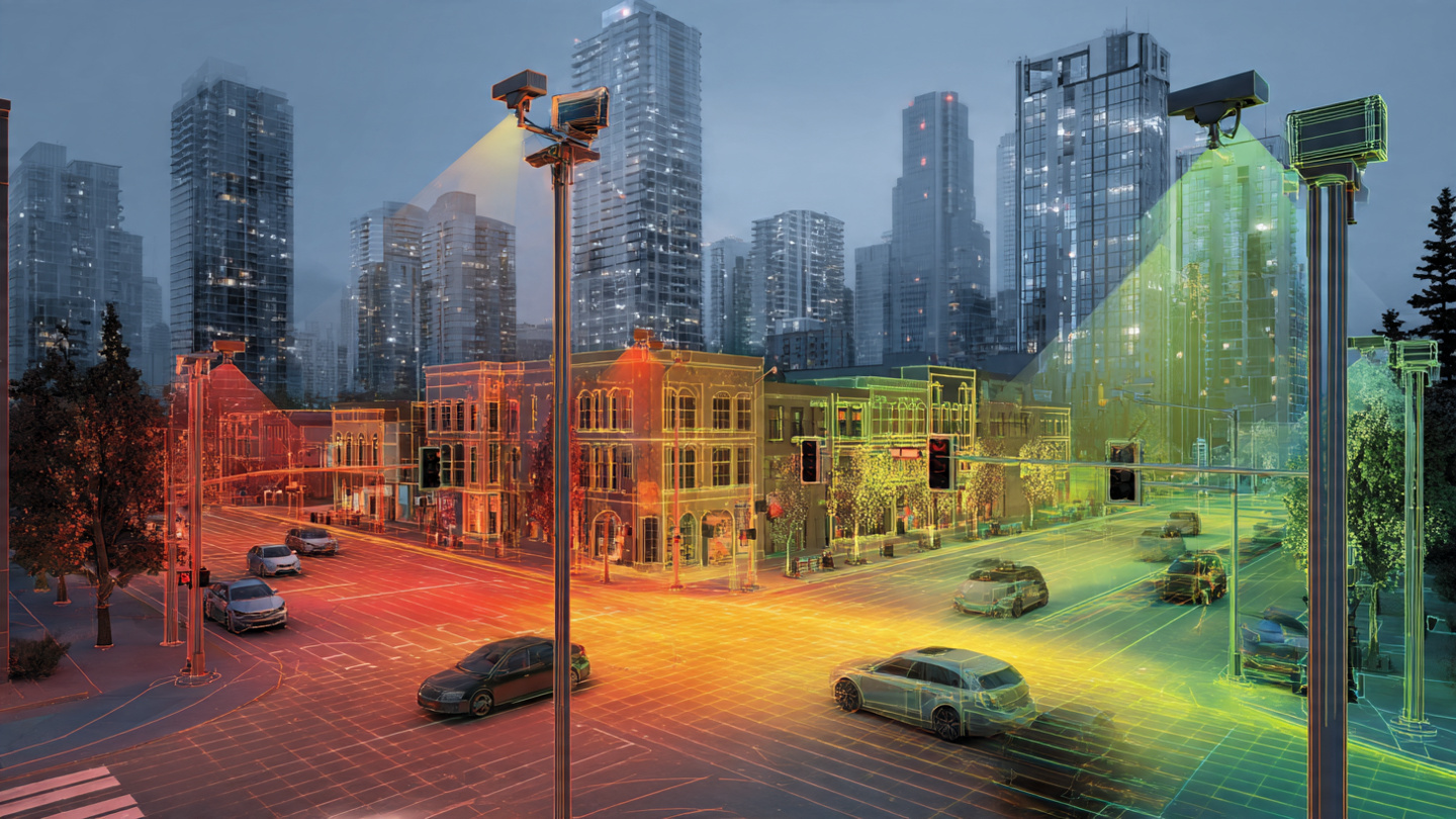
Disclosed is a system and method for estimating atmospheric particulate matter concentrations (PM2.5 and PM10) at street-level spatial resolution by analyzing visible-light extinction patterns captured by existing outdoor camera infrastructure. The system identifies stable visual reference targets at known distances within each camera's field of view, computes spectral contrast attenuation ratios across the visible band (red, green, blue channels), and derives scene-specific optical depth estimates using the Beer-Lambert-Bouguer law. A convolutional neural network trained on synchronized pairs of camera imagery and colocated federal reference method (FRM) monitor readings performs nonlinear calibration that accounts for relative humidity, solar geometry, aerosol composition variability, and camera-specific sensor response functions. The system operates at the edge on existing camera computing hardware, produces PM2.5 and PM10 estimates at 5-minute intervals per camera, and aggregates across camera networks to generate continuous spatial pollution maps at 100-meter resolution across urban areas. This transforms the estimated 85 million outdoor cameras already deployed in the United States into the densest ambient air quality monitoring network ever constructed, at zero incremental hardware cost.
Field of the Invention
This invention relates to environmental monitoring and urban sensing, specifically to the estimation of atmospheric particulate matter concentrations using image analysis of existing outdoor camera feeds combined with machine learning calibration against regulatory-grade reference instruments.
Background
Ambient particulate matter (PM2.5 and PM10) exposure causes an estimated 6.7 million premature deaths annually worldwide (Health Effects Institute, State of Global Air 2024), making it the single largest environmental health risk factor. In the United States, the EPA operates approximately 4,000 ambient air quality monitoring sites (EPA AMTIC), of which roughly 1,100 measure PM2.5. These stations cost $15,000-$50,000 each for federal reference method (FRM) instruments, plus $5,000-$10,000 annually for maintenance and calibration.
The resulting spatial coverage is grossly inadequate. A city like Los Angeles, spanning 1,302 km², operates approximately 20 PM2.5 monitors. Each monitor nominally "represents" 65 km² of urban area. Real particulate concentrations vary by factors of 2-5x within a single kilometer due to traffic corridors, construction sites, restaurant cooking exhaust, and topographic channeling effects documented by Apte et al. (Environmental Science & Technology, 2017), who measured 8x intra-urban variability in ultrafine particles across Oakland, California using mobile monitoring platforms.
Low-cost particulate sensors (PurpleAir PA-II at $229, Clarity Node-S at approximately $2,500) have proliferated, with over 40,000 PurpleAir units deployed globally as of 2025. However, these sensors suffer from well-documented limitations:
- Humidity interference: Light-scattering nephelometers overestimate PM2.5 by 30-300% at relative humidity above 60%, requiring correction factors that themselves introduce 15-25% uncertainty (Barkjohn et al., Atmospheric Measurement Techniques, 2019).
- Sensor drift: Plantower PMS5003 sensors, used in most consumer-grade monitors, exhibit 10-40% degradation over 12-18 months from optical chamber contamination (Zusman et al., Atmospheric Environment, 2020).
- Composition blindness: Scattering-based sensors cannot distinguish between hygroscopic sulfate aerosols, carbonaceous combustion particles, and mineral dust, which have different health effects and require different correction approaches.
Satellite-based aerosol optical depth (AOD) retrieval from instruments like MODIS and VIIRS provides global coverage but at 3-10 km spatial resolution and with temporal gaps due to cloud cover. Van Donkelaar et al. (Environmental Science & Technology, 2016) demonstrated that satellite AOD-to-PM2.5 conversion at ground level requires regional chemical transport model correction, introducing model-dependent bias of 20-40%.
Meanwhile, an estimated 85 million outdoor surveillance cameras operate across the United States (IFSEC Global, 2024), with over 1 billion globally. Traffic management systems in major US cities operate 10,000-50,000 cameras each. Every one of these cameras captures images that encode atmospheric optical properties. The gap in the art is a system that systematically extracts particulate matter estimates from this existing infrastructure, calibrated to regulatory-grade accuracy, operating in real time at the edge.
Detailed Description
1. Reference Target Identification and Registration
For each camera in the network, the system performs a one-time registration phase during which stable visual reference targets are identified at multiple known distances within the camera's field of view. Reference targets must satisfy three criteria: (a) fixed position (buildings, traffic signs, bridge structures, not trees or vehicles), (b) known distance from camera (computed via GIS coordinates of both camera and target, or measured via lidar survey), and (c) broadband spectral reflectance (light-colored surfaces preferred for maximum contrast sensitivity).
During registration, the algorithm employs SIFT (Scale-Invariant Feature Transform) keypoint detection to identify geometrically stable features, then tracks these features across 24 hours of imagery to reject transient objects. For each surviving reference target, the system records: pixel coordinates, physical distance from camera, approximate spectral reflectance class (high/medium/low, determined from daytime clear-sky imagery), and occlusion schedule (times when shadows, sun glare, or seasonal vegetation changes obscure the target).
A minimum of three reference targets at different distances (near: 50-200 m, mid: 200-500 m, far: 500-2000 m) is required per camera to enable multi-range optical depth estimation. Urban environments typically yield 15-30 viable targets per camera.
2. Visible-Light Extinction Measurement
Atmospheric extinction is measured by comparing the apparent contrast of reference targets against their clear-sky baseline. For each reference target at distance d, the system computes the contrast ratio C(d) in each color channel (R, G, B):
C(d) = |L_target - L_background| / L_background
where L_target and L_background are the luminance values of the target and adjacent sky or background region, respectively. Under the Beer-Lambert-Bouguer law, contrast decreases exponentially with distance and extinction coefficient:
C(d) = C₀ × exp(-b_ext × d)
where C₀ is the inherent contrast at zero distance and b_ext is the atmospheric extinction coefficient in units of inverse meters. By measuring C(d) at multiple known distances, the system solves for b_ext via weighted least-squares regression on log-transformed contrast ratios.
Extinction coefficient b_ext relates to PM2.5 mass concentration through the mass extinction efficiency (MEE), which depends on aerosol composition and relative humidity. Typical MEE values range from 3.0 m²/g for dry sulfate aerosol to 8.5 m²/g for aged urban haze at 80% RH (Hand and Malm, Atmospheric Environment, 2007).
Spectral decomposition across R, G, and B channels provides additional information about particle size distribution. Rayleigh scattering (proportional to λ⁻⁴) dominates for particles much smaller than visible wavelengths, while Mie scattering (approximately wavelength-independent) dominates for PM2.5-PM10 range particles. The ratio of blue-channel to red-channel extinction coefficients (the Ångström exponent proxy) distinguishes fine-mode (combustion, secondary organic) from coarse-mode (dust, sea salt) aerosol, enabling separate PM2.5 and PM10 estimation.
3. Neural Calibration Model
Raw extinction-to-PM conversion is confounded by multiple variables: relative humidity (hygroscopic growth increases scattering without changing mass), solar angle (forward scattering vs. backscattering geometry), aerosol composition (absorbing black carbon vs. scattering sulfate), camera auto-exposure and white balance adjustments, and lens contamination. A purely physical model cannot account for all these factors simultaneously.
The system therefore trains a convolutional neural network (CNN) that takes as input: (a) the multi-distance, multi-channel contrast ratio vector (3 distances × 3 channels = 9 features), (b) meteorological covariates from nearest weather station (temperature, relative humidity, wind speed, wind direction, solar irradiance), (c) temporal features (hour of day, day of year, for diurnal and seasonal patterns), and (d) camera metadata (lens focal length, sensor type, mounting height, compass bearing). The CNN output is PM2.5 and PM10 concentration estimates in μg/m³.
Training data is generated by synchronizing camera imagery with hourly readings from colocated FRM or FEM (federal equivalent method) monitors. A camera within 2 km of a regulatory monitor constitutes a training pair. The calibration dataset requires a minimum of 90 days spanning at least two seasons to capture the range of meteorological and aerosol conditions. Data augmentation includes synthetic camera degradation (lens blur, exposure noise, compression artifacts) to improve generalization across camera hardware variants.
Transfer learning enables calibration of cameras far from any regulatory monitor. A base model trained on the full network of colocated camera-monitor pairs captures general extinction-to-PM relationships. For cameras without nearby monitors, the base model is fine-tuned using: (a) spatial interpolation of PM values from surrounding monitors, (b) satellite AOD as a weak supervisory signal, and (c) periodic mobile reference colocation where a vehicle-mounted FRM instrument parks near the camera for 24-48 hours.
4. Edge Deployment Architecture
For deployment, the inference model is quantized to INT8 and compiled for deployment on the camera's existing computing hardware. Modern IP cameras typically include ARM Cortex-A series processors or dedicated video processing SoCs with sufficient compute for real-time inference:
- Axis ARTPEC-8: Quad-core ARM, 4 TOPS neural processing unit. Supports ONNX model deployment via Axis ACAP framework.
- Hikvision Falcon-G: Embedded AI chipset, 2 TOPS. DeepinView cameras support custom algorithm sideloading.
- NVIDIA Jetson Nano (retrofit): 472 GFLOPS GPU. Deployed as USB companion to legacy cameras without onboard compute.
The inference pipeline runs every 5 minutes (configurable). Each cycle: acquires a burst of 5 frames over 2 seconds (averaging reduces transient occlusion noise from vehicles and pedestrians), computes reference target contrast ratios, appends meteorological covariates from a local weather API, runs the calibration CNN, and publishes the PM2.5/PM10 estimate to a central aggregation service via MQTT over TLS. Total per-cycle compute: under 200 ms on ARTPEC-8 class hardware. Memory footprint: under 50 MB including model weights.
5. Spatial Aggregation and Map Generation
The central aggregation service receives PM estimates from all cameras in the network. Because each camera's estimate represents a line-of-sight averaged extinction measurement weighted toward the near-field (extinction contribution drops exponentially with distance), the effective "sensing footprint" of each camera is an elongated ellipse along the camera's viewing axis, with a half-power radius of approximately 200 meters. Overlapping footprints from cameras at intersections create a network of constrained observations.
Spatial interpolation employs ordinary kriging with an exponential variogram model. The variogram range parameter (typically 500-1500 m for urban PM2.5) is estimated empirically from the network's own data. Kriging produces both an interpolated PM2.5/PM10 surface and a spatially-varying uncertainty estimate. Grid resolution is 100 m × 100 m. In areas with camera density exceeding 5 per km² (typical for urban cores), the kriging uncertainty drops below ±3 μg/m³ for PM2.5.
The aggregation service exposes the interpolated map via a GeoJSON REST API, updated every 5 minutes, with endpoints for: current conditions (latest map), time-series at any grid point (hourly averages for past 30 days), and episodic event detection (wildfires, construction, traffic incidents that produce localized PM spikes exceeding 3σ above the spatial mean).
6. Self-Calibration and Drift Correction
Camera sensors degrade over time: lens surfaces accumulate grime, CMOS sensors develop hot pixels, and auto-exposure algorithms shift baselines. Without correction, these changes would be misinterpreted as atmospheric changes. The system employs three drift-mitigation strategies:
- Nighttime baseline reset: At 2:00-4:00 AM local time (minimal traffic aerosol), the system measures reference target contrast under near-background conditions. Systematic drift in nighttime contrast indicates camera hardware degradation, and the calibration model adjusts its camera-specific offset accordingly.
- Rain-wash calibration: During and immediately after rain events (detected via weather API), PM2.5 concentrations drop to near-background levels (typically below 5 μg/m³). The system uses these natural "clean air" events as calibration anchors, comparing camera-derived estimates against the expected post-rain baseline.
- Cross-camera consistency: Where multiple cameras view overlapping spatial regions, the system detects single-camera drift as deviation from the multi-camera consensus. A camera whose estimates diverge from its neighbors by more than 2σ for more than 48 hours is flagged for maintenance and its weight in the kriging interpolation is reduced to zero until corrected.
7. Figures Description
- Figure 1: System architecture showing camera network, edge inference nodes, MQTT aggregation, kriging interpolation, and GeoJSON API consumer applications including public health dashboards and routing engines.
- Figure 2: Reference target identification process: SIFT keypoint detection, 24-hour stability tracking, multi-distance target selection, and clear-sky baseline calibration for a representative urban intersection camera.
- Figure 3: Spectral contrast attenuation curves for red, green, and blue channels across six reference targets at distances of 80 m to 1,200 m, under PM2.5 concentrations of 8 μg/m³ (clean), 35 μg/m³ (moderate), and 150 μg/m³ (unhealthy). Demonstrates measurable contrast differences across the full EPA AQI range.
- Figure 4: Example 100-meter resolution PM2.5 map for a 25 km² urban area generated from 340 traffic cameras, showing localized hotspots near highway on-ramps, construction sites, and restaurant clusters, with kriging uncertainty contours overlaid.
- Figure 5: Transfer learning calibration architecture: base model trained on 200 colocated camera-monitor pairs, fine-tuned for remote cameras using spatial PM interpolation and mobile reference colocation.
Claims
- A system for estimating atmospheric particulate matter concentrations at street-level spatial resolution, comprising: a network of existing outdoor cameras, each with identified stable visual reference targets at known distances; an edge-deployed inference module at each camera that computes spectral contrast attenuation ratios across visible-light channels between reference targets and their backgrounds; and a neural calibration model that converts multi-distance, multi-channel contrast ratio vectors into PM2.5 and PM10 mass concentration estimates.
- The system of claim 1, wherein the neural calibration model is trained on synchronized pairs of camera imagery and readings from colocated federal reference method or federal equivalent method particulate monitors, and further incorporates meteorological covariates including relative humidity, temperature, wind speed, and solar geometry.
- The system of claim 1, wherein spectral decomposition across red, green, and blue color channels provides an Ångström exponent proxy that distinguishes fine-mode aerosol (PM2.5) from coarse-mode aerosol (PM10), enabling separate mass concentration estimates for each size fraction.
- The system of claim 1, further comprising a reference target registration module that employs scale-invariant feature detection and 24-hour temporal stability tracking to automatically identify fixed visual targets at near (50-200 m), mid (200-500 m), and far (500-2000 m) distances within each camera's field of view.
- The system of claim 1, further comprising a spatial aggregation service that receives PM estimates from multiple cameras, models each camera's sensing footprint as a line-of-sight weighted ellipse, and performs kriging interpolation to generate continuous particulate matter concentration maps with spatially-varying uncertainty at configurable grid resolution.
- The system of claim 1, further comprising a self-calibration module that detects camera hardware drift using nighttime baseline contrast measurements, post-rain near-background calibration anchors, and cross-camera consistency checks against spatially neighboring cameras.
- A method for converting existing outdoor camera infrastructure into an ambient air quality monitoring network, comprising: performing one-time registration of stable visual reference targets at known distances within each camera's field of view; periodically computing multi-channel contrast attenuation between reference targets and backgrounds; applying a learned calibration model that maps contrast attenuation vectors and meteorological covariates to PM2.5 and PM10 mass concentrations; and spatially interpolating per-camera estimates to produce continuous urban-scale particulate matter maps.
- The method of claim 7, wherein a base calibration model trained on cameras colocated with regulatory monitors is transferred to cameras without nearby monitors via fine-tuning using spatially-interpolated PM values, satellite aerosol optical depth as a weak supervisory signal, and periodic mobile reference monitor colocation.
- The method of claim 7, further comprising episodic event detection wherein localized PM concentrations exceeding a configurable threshold above the spatial mean trigger source-attribution analysis based on the spatial pattern and temporal evolution of the plume across multiple camera observations.
- The system of claim 1, wherein inference is performed entirely at the camera edge, the quantized model occupies less than 50 MB of memory, inference completes in less than 500 milliseconds per cycle, and only scalar PM estimates are transmitted to the aggregation service, preserving privacy by never transmitting camera imagery off-device.
- The system of claim 5, wherein the aggregation service exposes a GeoJSON REST API providing current conditions, historical time-series at any grid point, and episodic event alerts, enabling integration with public health dashboards, air quality routing engines, and urban planning tools.
- The method of claim 7, wherein the system is deployable across heterogeneous camera hardware from different manufacturers without retraining the base model, using camera-specific fine-tuning on as few as 7 days of colocated reference data to adapt the calibration for sensor response function, lens characteristics, and mounting geometry differences.
Prior Art References
- Health Effects Institute — State of Global Air 2024 — 6.7 million annual deaths from PM exposure
- EPA AMTIC — Federal air monitoring site counts and network descriptions
- Apte et al., Environmental Science & Technology 2017 — 8x intra-urban variability in ultrafine particles, Oakland mobile monitoring
- Barkjohn et al., Atmospheric Measurement Techniques 2019 — PurpleAir humidity correction factors and residual uncertainty
- Zusman et al., Atmospheric Environment 2020 — Plantower PMS5003 sensor degradation over 12-18 months
- Van Donkelaar et al., Environmental Science & Technology 2016 — Satellite AOD-to-PM2.5 conversion methodology and limitations
- Hand and Malm, Atmospheric Environment 2007 — Mass extinction efficiency values by aerosol type and humidity
- Xie et al., Applied Optics 2003 — Visibility estimation from digital camera images using contrast attenuation
- Liu et al., Environmental Pollution 2018 — Webcam-based visibility monitoring and PM2.5 correlation in Chinese megacities
- IFSEC Global — Global surveillance camera market estimates (85M+ US outdoor cameras)
- Li et al., Journal of Geophysical Research: Atmospheres 2020 — Ground-based camera networks for aerosol optical depth retrieval
- Guo et al., Remote Sensing of Environment 2014 — Linking ground-level PM2.5 with satellite AOD at high spatial resolution
- TensorFlow Lite — On-device ML runtime for edge inference
- MQTT Protocol — Lightweight IoT messaging standard for sensor data aggregation