System and Method for Continuous Estimation of Lithium-Ion Battery Cell Internal Temperature Distribution Using Multi-Frequency Electrochemical Impedance Spectroscopy Superimposed on Operational Current with Physics-Constrained Neural Network Inversion on Standard Battery Management System Hardware

Abstract

Disclosed is a system and method for continuously estimating the internal radial temperature distribution of lithium-ion battery cells during normal charge and discharge operations without embedded thermocouples, fiber-optic sensors, or dedicated laboratory impedance analyzers. The system superimposes low-amplitude multi-frequency AC perturbation signals (5 mV–20 mV RMS, logarithmically spaced from 0.1 Hz to 10 kHz) onto the operational DC current using the existing MOSFET gate drive circuitry of standard battery management system (BMS) analog front-end integrated circuits (e.g., Texas Instruments BQ79616, Analog Devices ADBMS6830). The resulting voltage response is sampled by the BMS ADC and processed through a discrete Fourier transform to extract the complex impedance spectrum Z(f) = Z'(f) + jZ''(f). Because different electrochemical processes dominate at different frequencies, and each process has a distinct Arrhenius temperature dependence, the impedance spectrum encodes temperature information at multiple effective "depths" within the cell: ohmic resistance R₀ (dominated by electrolyte ionic conductivity, activation energy E_a ≈ 0.15–0.25 eV) responds primarily to the bulk average temperature; charge transfer resistance R_ct (activation energy E_a ≈ 0.4–0.7 eV) reflects electrode-electrolyte interface temperature; and solid-state diffusion impedance Z_W (activation energy E_a ≈ 0.3–0.5 eV) correlates with particle-interior temperature. A physics-constrained neural network (68,000 parameters, 140 KB quantized INT8) running on the BMS microcontroller inverts the measured impedance spectrum by embedding Arrhenius kinetics and a lumped radial thermal model as differentiable network layers, outputting estimated temperatures at three radial positions (core, mid-radius, surface) with a target accuracy of ±1.5°C and 10-second temporal resolution. The system detects internal hot spots and thermal runaway precursors 30–120 seconds earlier than surface-mounted thermistors, within the hardware and power budget of production BMS platforms at zero additional bill-of-materials cost.

Field of the Invention

This invention relates to thermal monitoring of lithium-ion battery systems, specifically to methods for estimating the spatially-resolved internal temperature of battery cells using electrochemical impedance analysis performed on existing battery management system hardware with physics-informed machine learning inversion.

Background

Lithium-ion battery thermal management is the primary engineering constraint in electric vehicle (EV) design, grid-scale energy storage, and consumer electronics. The National Highway Traffic Safety Administration recorded 52 EV battery fire incidents in the US in 2024, while the global count exceeded 300 events per year across all applications. Internal cell temperatures during thermal runaway onset exceed surface temperatures by 20–50°C, and surface-mounted temperature sensors (NTC thermistors, the universal standard in production BMS) detect the thermal anomaly only after heat has conducted through the cell casing. For a cylindrical 21700 cell with a radial thermal conductivity of approximately 1 W/m·K, the thermal time constant from core to surface is 30–120 seconds, meaning surface sensors are inherently late by this margin.

Current approaches to measuring or estimating internal battery temperature suffer from fundamental limitations:

• Surface-mounted NTC thermistors: The industry standard. Every production BMS uses 10 kΩ NTC thermistors (±1°C accuracy) bonded to the cell exterior or module casing. Cost: $0.05–$0.15 per sensor. They measure surface temperature only, which lags core temperature by 30–120 seconds depending on cell geometry and cooling configuration. During fast charging at 2C rate, the core-to-surface gradient in a 21700 cell reaches 8–15°C (Forgez et al., Journal of Power Sources, 2010). This gradient is invisible to surface sensors.
• Embedded thermocouples: Research groups at NREL (Keyser et al., 2015) and others have inserted micro-thermocouples into cell interiors through modified cell casings. Provides direct measurement with ±0.5°C accuracy, but destroys the cell seal, introduces contamination risks, and is incompatible with production manufacturing. Useful for laboratory validation only.
• Fiber Bragg grating sensors: Nascimento et al. (Journal of Power Sources, 2020) demonstrated distributed temperature sensing inside pouch cells using fiber-optic gratings with 1 mm spatial resolution and ±0.1°C accuracy. Requires optical fiber routed through the cell (incompatible with production), an interrogator unit ($5,000–$20,000), and is mechanically fragile. Strictly a research tool.
• Electrochemical model-based estimation: Lin et al. (Journal of the Electrochemical Society, 2020) used a reduced-order electrochemical-thermal model coupled with an Extended Kalman Filter to estimate internal temperature from terminal voltage measurements. Achieves ±2–4°C accuracy but requires computationally expensive model integration (>100 ms per step on typical BMS microcontrollers), careful parameterization for each cell chemistry, and degrades as cells age because the electrochemical model parameters drift.
• Laboratory EIS-based temperature estimation: Koleti et al. (EES Batteries, 2024) demonstrated that EIS features, particularly charge transfer resistance R_ct, can estimate internal cell temperature with ±0.41°C accuracy for cylindrical cells. However, their method requires a dedicated potentiostat/galvanostat (e.g., BioLogic SP-300, $25,000+), measurement at rest (no load current), and offline processing. It is not compatible with real-time BMS operation. Xu et al. (Journal of Energy Storage, 2024) extended the approach to sodium-ion cells using machine learning, achieving 1.086°C average error, but still required laboratory EIS equipment.
• Under-load EIS: Srinivasan et al. (Journal of the Electrochemical Society, 2019) explored performing EIS measurements during battery discharge, demonstrating feasibility but noting significant artifacts from the DC current bias. They did not address temperature distribution estimation, physics-constrained inversion, or deployment on standard BMS hardware.

The gap in the art is a complete system that: (a) performs impedance spectroscopy using the existing hardware in production BMS ICs, without dedicated analog front-end additions; (b) operates during normal charge and discharge with appropriate artifact compensation; (c) extracts spatially-resolved internal temperature information by exploiting the frequency-dependent thermal sensitivity of different electrochemical processes; (d) uses physics-constrained machine learning for robust inversion that generalizes across cell aging states; and (e) runs on the standard BMS microcontroller within real-time computational constraints.

Detailed Description

1. Impedance Measurement Using Standard BMS Hardware

Modern BMS analog front-end (AFE) ICs include programmable cell-balancing circuits capable of sinking or sourcing small currents through integrated MOSFETs or external balancing resistors. The TI BQ79616 provides per-cell balancing with programmable current (0–200 mA) and 16-bit ADC sampling at up to 976 SPS. The Analog Devices ADBMS6830 offers similar capabilities with 18-bit resolution and on-chip diagnostic functions. These circuits, designed for passive cell balancing, can be repurposed to inject small AC perturbation signals by rapidly toggling the balancing MOSFET with a programmed waveform.

The perturbation signal is a multi-sine waveform comprising 8–12 logarithmically-spaced frequencies from 0.1 Hz to 10 kHz, with individual frequency amplitudes of 5–20 mV RMS (cell voltage perturbation). This amplitude is small enough to satisfy the linearity requirement for impedance spectroscopy (voltage perturbation < 1% of cell OCV) while producing measurable current perturbation above the ADC noise floor. The composite multi-sine signal excites all frequencies simultaneously, allowing a complete impedance spectrum to be acquired in a single measurement window of 10 seconds (limited by the period of the lowest frequency component at 0.1 Hz).

The BMS ADC simultaneously samples the cell voltage response at 1 kSPS (adequate for frequencies up to 500 Hz per Nyquist; higher frequencies use the AFE's built-in high-speed comparator with time-stamped threshold crossings for phase measurement). A discrete Fourier transform (DFT) computed at the exact excitation frequencies extracts the complex impedance Z(f) at each frequency. Because the excitation frequencies are known precisely (generated by the same microcontroller clock), the DFT reduces to a set of dot products between the sampled voltage and stored reference sinusoids, requiring approximately 24,000 multiply-accumulate operations per measurement window on an ARM Cortex-M4F at 80 MHz (under 1 ms of computation).

2. DC Bias Artifact Compensation

Unlike laboratory EIS measurements performed at rest, this system operates during normal charge and discharge when a DC current bias of 0.1–5C is flowing through the cell. The DC bias creates two artifacts that must be compensated:

1. Nonlinear distortion: At high DC bias currents, the Butler-Volmer kinetics become asymmetric, and the small-signal impedance depends on the operating point. The system compensates by measuring the DC operating point (current and voltage) at the start of each measurement window and applying a first-order bias correction derived from the cell's Butler-Volmer parameters: R_ct_corrected = R_ct_measured × (α_a + α_c) × F × η / (RT × sinh((α_a + α_c) × F × η / (2RT))), where α_a and α_c are anodic and cathodic transfer coefficients, F is Faraday's constant, η is the overpotential, R is the gas constant, and T is the current temperature estimate (iteratively refined).
2. Spectral leakage from DC drift: The cell voltage changes during the 10-second measurement window due to state-of-charge (SoC) variation and thermal drift. At 1C discharge, the OCV changes by approximately 3–10 mV over 10 seconds (depending on the SoC region and cell chemistry). This manifests as low-frequency spectral content that contaminates the impedance measurement below ~1 Hz. The system applies a piecewise-linear detrending filter to the voltage time series before DFT computation, removing the slowly-varying DC component while preserving the AC perturbation response.

3. Frequency-Dependent Thermal Sensitivity of Electrochemical Processes

The key physical insight enabling spatial temperature resolution is that different electrochemical processes dominate the impedance at different frequencies, and each process has a distinct Arrhenius-type temperature dependence with a different activation energy. This creates a natural "depth selectivity" because the processes probing the cell interior (solid-state diffusion) are separable in frequency from those at the electrode surface (charge transfer) and the bulk electrolyte (ohmic conduction):

• High frequency (1–10 kHz): Ohmic resistance R₀. Dominated by electrolyte ionic conductivity, current collector resistance, and contact resistances. The electrolyte conductivity of LiPF₆ in EC:DMC follows a modified Arrhenius relationship with activation energy E_a ≈ 0.15–0.25 eV (Valøen and Reimers, Journal of the Electrochemical Society, 2005). Temperature coefficient: approximately −0.5% to −1.5% per °C increase. This resistance reflects the volume-averaged temperature of the electrolyte along the current path, which for a cylindrical cell with radial thermal gradient correlates most strongly with the temperature at the mid-radius position.
• Mid frequency (1–1,000 Hz): Charge transfer resistance R_ct. Governed by the electrode-electrolyte interfacial kinetics described by Butler-Volmer equation. The exchange current density i₀ follows Arrhenius kinetics with E_a ≈ 0.4–0.7 eV for graphite anodes and 0.5–0.8 eV for NMC/NCA/LFP cathodes (Ecker et al., Journal of the Electrochemical Society, 2015). Temperature coefficient: approximately −2% to −5% per °C for R_ct. This large thermal sensitivity makes R_ct the most information-rich feature for temperature estimation. Because charge transfer occurs at the electrode-electrolyte interface (near the cell surface for the outermost electrode), R_ct reflects a weighted average that is biased toward the electrode-surface temperature.
• Low frequency (0.1–1 Hz): Solid-state diffusion impedance Z_W. Governed by lithium-ion diffusion within the active material particles. The solid-state diffusion coefficient D_s follows Arrhenius kinetics with E_a ≈ 0.3–0.5 eV for graphite and 0.4–0.6 eV for NMC (Gao et al., Electrochimica Acta, 2017). The Warburg impedance Z_W ∝ 1/√(D_s) ∝ exp(E_a / (2kT)), giving a temperature coefficient of approximately −1.5% to −3% per °C. Because solid-state diffusion occurs within the active material particles throughout the electrode thickness, and the thickest electrodes are in the innermost windings of a cylindrical cell (where the jelly roll is most tightly wound), the diffusion impedance preferentially samples the core temperature.

The ratio of R_ct to R₀, and of Z_W to R₀, therefore encodes information about the temperature gradient. In a thermally uniform cell, these ratios are determined solely by the cell's electrochemistry. When a radial temperature gradient exists (core hotter than surface), the diffusion impedance Z_W decreases relative to R₀ more than expected for a uniform cell at the surface temperature, because the core is hotter. The magnitude of this anomaly is proportional to the temperature gradient.

4. Physics-Constrained Neural Network Architecture

A purely data-driven approach to inverting the impedance spectrum for temperature would require extensive training data covering all combinations of temperature distribution, SoC, state of health (SoH), and C-rate, making it brittle and poorly generalizing. Instead, the system embeds the known physics as differentiable constraints within the neural network architecture:

• Input layer: 24 features from the measured impedance spectrum: real and imaginary components at 12 frequencies (Z'(f_i), Z''(f_i) for i = 1..12), plus 4 auxiliary inputs (DC current, cell voltage, estimated SoC from coulomb counting, and surface NTC temperature if available).
• Physics embedding layer (differentiable Arrhenius): A custom layer that takes the raw impedance features and decomposes them into physically meaningful parameters using a learnable equivalent circuit fitting. The layer outputs estimates of R₀, R_ct (anode), R_ct (cathode), C_dl (anode), C_dl (cathode), and σ_W (Warburg coefficient). Each parameter is then passed through a differentiable Arrhenius inversion: T_estimated = E_a / (k × ln(R_ref / R_measured)), where E_a is a learnable activation energy (initialized from literature values but refined during training), k is Boltzmann's constant, and R_ref is a learnable reference resistance at a reference temperature.
• Thermal model layer (differentiable lumped radial model): The three temperature estimates from the Arrhenius inversions (T_core_est from Z_W, T_mid_est from R₀, T_surface_est from R_ct) are passed through a differentiable 3-node radial thermal model that enforces physical consistency: dT_core/dt = (Q_gen − (T_core − T_mid)/R_th_1) / C_th_1, dT_mid/dt = ((T_core − T_mid)/R_th_1 − (T_mid − T_surface)/R_th_2) / C_th_2. Here R_th_1 and R_th_2 are learnable thermal resistances and C_th_1 and C_th_2 are learnable thermal capacitances, initialized from cell geometry and material properties. This layer rejects physically impossible temperature distributions (e.g., surface hotter than core during discharge without external heating).
• Residual correction block: Two dense layers (64 neurons, ReLU activation) that learn to correct systematic errors in the physics-based estimates arising from model simplifications (e.g., contact resistance variation with aging, SEI layer growth effects on R_ct). The correction is additive and bounded to ±5°C via a scaled tanh activation, preventing the data-driven component from overriding the physics.
• Output layer: Three temperature outputs (T_core, T_mid, T_surface) and a scalar "thermal gradient severity" index (0–100 scale) derived from (T_core − T_surface) normalized by a chemistry-dependent thermal runaway onset threshold.

Total parameter count: approximately 68,000. Quantized to INT8 using TensorFlow Lite for Microcontrollers: 140 KB model size. Inference time on ARM Cortex-M4F at 80 MHz: approximately 8 ms per 10-second measurement window. Memory footprint: 48 KB SRAM (within the 256 KB typical of BMS-grade microcontrollers such as the STM32L4 series).

5. Training Data Generation

The physics-constrained architecture reduces data requirements compared to purely data-driven approaches, but training data is still needed to calibrate the learnable parameters and the residual correction block:

1. Electrochemical-thermal simulation: A pseudo-two-dimensional (P2D) electrochemical model (Doyle, Fuller, Newman, 1993) coupled with a 2D axisymmetric thermal model, implemented in COMSOL Multiphysics or PyBaMM (pybamm.org), generates synthetic impedance spectra for cylindrical (18650, 21700, 4680) and prismatic cell geometries across a parameter space of: temperatures (−20°C to +60°C surface, 0 to +30°C core-surface gradient), SoC (5%–95% in 5% steps), C-rate (0C to 5C), and SoH (100%–70% capacity retention). The P2D model computes the linearized impedance response at each frequency by applying a small sinusoidal perturbation to the steady-state solution. This generates approximately 200,000 labeled training examples per cell geometry.
2. Laboratory validation with embedded sensors: A calibration dataset is generated using cells instrumented with internal micro-thermocouples (K-type, 80 µm diameter, inserted through the negative terminal crimp following the procedure of Keyser et al., 2015). Simultaneous EIS measurements using a research-grade potentiostat provide ground-truth impedance spectra paired with ground-truth internal temperatures. These instrumented cells are cycled across the full operational envelope to generate approximately 5,000 high-fidelity validation examples.
3. Transfer learning for cell chemistry: The physics embedding layer (Arrhenius inversions, thermal model) transfers well across cell chemistries because the underlying physics is universal. Only the learnable activation energies, reference resistances, and thermal model parameters need re-calibration for each new chemistry. This is accomplished through fine-tuning on 500–1,000 chemistry-specific simulation examples, taking approximately 30 minutes on a standard GPU.

6. Aging Adaptation

Battery impedance increases with aging due to solid electrolyte interphase (SEI) growth, loss of lithium inventory, and loss of active material. These changes could confound temperature estimation if not accounted for. The system adapts to aging through two mechanisms:

1. Baseline tracking: During periods of thermal equilibrium (cell at rest for >30 minutes, surface temperature stable to ±0.5°C), the system measures a reference impedance spectrum and updates the baseline parameters (R₀_ref, R_ct_ref, σ_W_ref) used in the Arrhenius inversion layer. The surface NTC temperature during this calibration provides the ground-truth temperature for the thermally-uniform cell. This self-calibration occurs automatically during overnight parking for EVs or during standby periods for stationary storage.
2. Physics-based SoH decoupling: The Arrhenius relationship predicts specific functional forms for how each impedance component changes with temperature. Aging changes the pre-exponential factor (R_ref) but not the activation energy (E_a) for each process. The physics embedding layer separates these effects: R_measured(T) = R_ref(SoH) × exp(E_a / (kT)), where R_ref(SoH) is updated during calibration and E_a is learned during initial training and held fixed. This separation means that aging-induced impedance increases do not bias the temperature estimate.

7. Thermal Runaway Precursor Detection

The system's ability to estimate core temperature independently of surface temperature enables early detection of thermal runaway precursors. The onset of thermal runaway in NMC/NCA cathode materials begins with SEI decomposition at approximately 90–120°C, followed by cathode-electrolyte reactions at 150–200°C (Feng et al., Journal of Power Sources, 2012). These exothermic reactions initially occur at the cell core (hottest point) and propagate outward.

The system detects three precursor signatures in the impedance spectrum:

1. Anomalous core-surface gradient acceleration: During normal operation, the core-surface gradient changes smoothly with C-rate. An accelerating gradient (d²ΔT/dt² > 0) at constant or decreasing C-rate indicates an internal heat source (self-heating reaction). The thermal model layer detects this as a deviation from the predicted gradient trajectory.
2. SEI decomposition impedance signature: SEI decomposition releases gaseous products (ethylene, CO₂) that create gas bubbles at the electrode-electrolyte interface, causing a characteristic increase in the high-frequency impedance noise floor and a broadening of the mid-frequency semicircle in the Nyquist plot. A dedicated anomaly detection head on the neural network monitors the residual between measured and predicted impedance spectra, flagging deviations exceeding 3σ of the normal operating envelope.
3. Rapid ohmic resistance increase: Gas generation from early decomposition reactions reduces the effective electrolyte contact area, causing R₀ to increase faster than the Arrhenius prediction. The ratio R₀_measured / R₀_Arrhenius_predicted exceeds 1.0 when gas evolution begins, providing a chemistry-independent early warning signal.

The system issues a thermal warning when any precursor signature is detected, providing an estimated 30–120 seconds of advance warning compared to surface-mounted thermistors. For a 21700 cell at 1C discharge with an internal short circuit generating 5 W of localized heating, the system detects the anomaly when the core temperature reaches approximately 65°C (surface still at 45°C), compared to surface NTC detection at approximately 55°C surface temperature (core already at 90°C).

8. SoC Dependence Compensation

Battery impedance depends on both temperature and SoC, creating a cross-coupling that must be resolved. The charge transfer resistance R_ct varies by 2–5× across the SoC range for typical NMC cathodes (minimum near 50% SoC, increasing at extremes). This SoC dependence has a different functional form than the temperature dependence: R_ct(SoC) is governed by the lithium concentration at the electrode surface (Butler-Volmer kinetics), while R_ct(T) follows Arrhenius kinetics.

The physics embedding layer decouples these effects through a factored representation: R_ct(T, SoC) = R_ct_T(T) × f_SoC(SoC), where f_SoC is a learnable SoC correction function parameterized as a 5th-order Chebyshev polynomial. The SoC estimate comes from the BMS coulomb counter (available on all production BMS ICs). During the baseline calibration (thermal equilibrium), the system measures R_ct at the current SoC and temperature, providing a joint calibration point that anchors both the temperature and SoC correction functions.

9. Multi-Cell Pack-Level Deployment

In production EV battery packs containing 96–200+ series-connected cells (e.g., Tesla 4680 structural pack: ~400 cells in series-parallel), the BMS AFE monitors all cells sequentially through a daisy-chained communication bus (SPI or isoSPI). The impedance measurement system time-multiplexes across cells, measuring one cell per 10-second window and cycling through the entire pack in 15–35 minutes. Cells identified as thermally critical (highest gradient severity index or fastest gradient rate of change) are prioritized for more frequent measurement.

The pack-level controller aggregates individual cell temperature distribution estimates into a 3D thermal map of the entire pack, enabling: (a) identification of cooling system hot spots (cells receiving insufficient coolant flow); (b) detection of cell-to-cell thermal imbalance that accelerates differential aging; (c) C-rate limiting based on the hottest cell's core temperature rather than the hottest surface temperature; and (d) preemptive thermal management adjustments (increasing coolant flow, reducing charge rate) before surface temperatures indicate a problem.

10. Figures Description

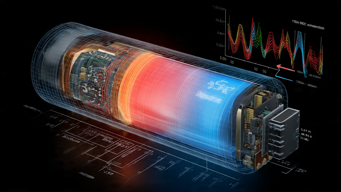
• Figure 1: Block diagram showing the signal flow from multi-sine perturbation generation through the BMS balancing MOSFET, to cell voltage response sampling by the BMS ADC, DFT extraction of the impedance spectrum, and physics-constrained neural network inversion to produce the three-point radial temperature profile.
• Figure 2: Nyquist plot (−Z'' vs Z') showing simulated impedance spectra for a 21700 NMC cell at three thermal conditions: (a) thermally uniform at 25°C, (b) thermally uniform at 45°C, and (c) gradient condition with core at 45°C and surface at 25°C. Annotations highlight the distinct changes in R₀ (high-frequency intercept), R_ct (mid-frequency semicircle diameter), and Z_W (low-frequency tail slope) for each condition.
• Figure 3: Architecture of the physics-constrained neural network showing the input feature vector, physics embedding layer (equivalent circuit decomposition → Arrhenius inversion), thermal model layer (3-node radial lumped model), residual correction block, and output heads for T_core, T_mid, T_surface, and thermal gradient severity index.
• Figure 4: Time-series comparison of estimated core temperature (from impedance system) versus measured core temperature (from embedded thermocouple) and surface NTC temperature during a simulated internal short circuit event, illustrating the 30–120 second early warning advantage.

Claims

1. A system for estimating the internal temperature distribution of a lithium-ion battery cell, comprising: a battery management system analog front-end integrated circuit connected to the cell; a perturbation signal generator that superimposes a multi-frequency AC signal onto the cell's operational current using the analog front-end's existing cell-balancing circuitry; an analog-to-digital converter sampling the cell voltage response; a digital signal processor computing the complex impedance spectrum at the perturbation frequencies; and a machine learning model that inverts the impedance spectrum to estimate temperatures at two or more radial positions within the cell.
2. The system of claim 1, wherein the multi-frequency AC signal is a multi-sine waveform comprising 4–16 logarithmically-spaced frequencies between 0.01 Hz and 100 kHz, with individual frequency amplitudes of 1–50 mV RMS.
3. The system of claim 1, wherein the machine learning model includes a physics embedding layer that decomposes the measured impedance into electrochemical parameters and applies Arrhenius-type thermal inversion to each parameter using learnable activation energies and reference resistances.
4. The system of claim 3, wherein the physics embedding layer includes a differentiable lumped radial thermal model that constrains the estimated temperature distribution to be physically consistent with heat conduction equations, rejecting temperature estimates that violate thermal energy conservation.
5. The system of claim 1, wherein the machine learning model further includes a bounded residual correction block comprising one or more dense neural network layers with output bounded to a predetermined range, correcting systematic errors in the physics-based temperature estimates without overriding the physical constraints.
6. The system of claim 1, further comprising a DC bias compensation module that corrects the measured impedance for nonlinear distortion and spectral leakage arising from the DC current flowing through the cell during normal charge or discharge operations.
7. The system of claim 1, further comprising a baseline calibration module that measures a reference impedance spectrum during periods of thermal equilibrium and updates the Arrhenius reference parameters to account for cell aging without biasing the temperature estimate.
8. The system of claim 1, further comprising a thermal runaway precursor detection module that monitors for: anomalous core-surface temperature gradient acceleration at constant or decreasing C-rate; impedance spectral signatures consistent with SEI decomposition gas evolution; and ohmic resistance increases exceeding the Arrhenius prediction for the estimated temperature.
9. A method for estimating internal battery cell temperature, comprising: generating a multi-frequency AC perturbation signal using existing cell-balancing circuitry of a battery management system; superimposing said perturbation signal onto the cell's operational charge or discharge current; sampling the cell's voltage response; computing the complex impedance at each perturbation frequency; decomposing the impedance spectrum into electrochemical parameters corresponding to processes at different spatial locations within the cell; applying Arrhenius-type thermal inversion to each parameter to obtain spatially-weighted temperature estimates; and constraining said estimates using a radial thermal model to produce a physically consistent internal temperature profile.
10. The method of claim 9, further comprising: factoring the SoC dependence of each impedance parameter from its temperature dependence using a learnable SoC correction function parameterized as a polynomial, where the SoC estimate is provided by the battery management system's coulomb counter.
11. The method of claim 9, further comprising: time-multiplexing impedance measurements across multiple cells in a battery pack; aggregating individual cell temperature distribution estimates into a three-dimensional thermal map; and prioritizing measurement frequency for cells exhibiting the highest thermal gradient severity or fastest gradient rate of change.
12. The system of claim 1, wherein the machine learning model is quantized to 8-bit integer precision and deployed on the battery management system's microcontroller, performing inference within 20 milliseconds per measurement window using less than 256 KB of SRAM.

Implementation Notes

A minimum viable implementation targets a single 21700 NMC cell monitored by a TI BQ79616 or Analog Devices ADBMS6830 AFE with an STM32L4 series microcontroller. The multi-sine perturbation is generated by PWM-modulating the cell balancing MOSFET at frequencies determined by the perturbation schedule, with the PWM carrier frequency set 10× above the highest impedance measurement frequency to ensure adequate signal purity. Initial model training uses PyBaMM P2D simulations for 21700 NMC/graphite chemistry, validated against 10 cells instrumented with embedded thermocouples at NREL-style insertion points. The trained model is exported via TensorFlow Lite for Microcontrollers and deployed as a firmware update, requiring no hardware changes to the existing BMS board. For automotive deployment, the system integrates with the BMS CAN bus to report core, mid-radius, and surface temperature estimates alongside the existing surface NTC reading, enabling the thermal management controller to use the more informative internal temperature data for cooling decisions and charge rate limiting. The zero-BOM-cost nature of this approach makes it deployable as a firmware update to any BMS platform using compatible AFE ICs, potentially retrofittable to vehicles already in the field through over-the-air (OTA) update.

Prior Art References

1. Koleti et al., EES Batteries (RSC), 2024 — Sensor-less EIS-based internal temperature estimation using DRT and Arrhenius modeling (±0.41°C cylindrical, ±2.22°C pouch; laboratory equipment only)
2. Xu et al., Journal of Energy Storage, 2024 — ML-based internal temperature estimation for sodium-ion batteries using EIS features (1.086°C average error; laboratory equipment)
3. Srinivasan et al., Journal of the Electrochemical Society, 2019 — Under-load EIS feasibility for temperature estimation (DC bias artifacts characterized but not resolved for production BMS)
4. Keyser et al., Journal of the Electrochemical Society, 2015 — Internal thermocouple insertion technique for cylindrical cells (laboratory validation method)
5. Nascimento et al., Journal of Power Sources, 2020 — Fiber Bragg grating distributed internal temperature sensing in pouch cells
6. Lin et al., Journal of the Electrochemical Society, 2020 — Electrochemical-thermal model with EKF for internal temperature estimation
7. Valøen and Reimers, Journal of the Electrochemical Society, 2005 — LiPF₆ electrolyte conductivity Arrhenius parameters
8. Ecker et al., Journal of the Electrochemical Society, 2015 — Parameterization of NMC/graphite cell equivalent circuit elements including temperature-dependent charge transfer kinetics
9. Gao et al., Electrochimica Acta, 2017 — Solid-state lithium diffusion coefficient Arrhenius parameters in NMC and graphite electrodes
10. Feng et al., Journal of Power Sources, 2012 — Thermal runaway mechanism characterization for NMC cathode materials
11. Forgez et al., Journal of Power Sources, 2010 — Core-to-surface temperature gradient measurements in cylindrical Li-ion cells during fast charge/discharge
12. Doyle, Fuller, Newman, Journal of the Electrochemical Society, 1993 — Pseudo-two-dimensional electrochemical model for lithium-ion batteries
13. PyBaMM — Open-source Python Battery Mathematical Modelling framework
14. Texas Instruments BQ79616 — 16-cell BMS AFE with integrated ADC and cell balancing
15. Analog Devices ADBMS6830 — 18-cell BMS AFE with high-accuracy ADC and diagnostic functions
16. TensorFlow Lite for Microcontrollers — Edge ML inference runtime for resource-constrained devices
17. STM32L4 Series — ARM Cortex-M4F microcontrollers used in production BMS designs